What is randomness? And how can we generate it? Both questions — the first mathematical, the second technological — have profound implications in many of today’s industries and our everyday lives.
Imagine that we wanted to make a random list of 0s and 1s. This list could be used to protect your medical records as a keyword, could ensure that a lottery is trustworthy, or could encrypt a digital letter to your long-lost half-step-brother-in-law. To make this list, maybe you use the classic coin-flip method: write down a 1 every time the coin lands heads-up and a 0 otherwise. Or maybe instead, you time the decay of the radioactive cesium that you stole from the lab. Is one of these methods better than the other; does it even matter? Yes, on both counts.
Let’s explore the principles of randomness together, and some new results from Quandela that generate certifiable randomness according to the laws of quantum mechanics.
Part 2: Generating randomness
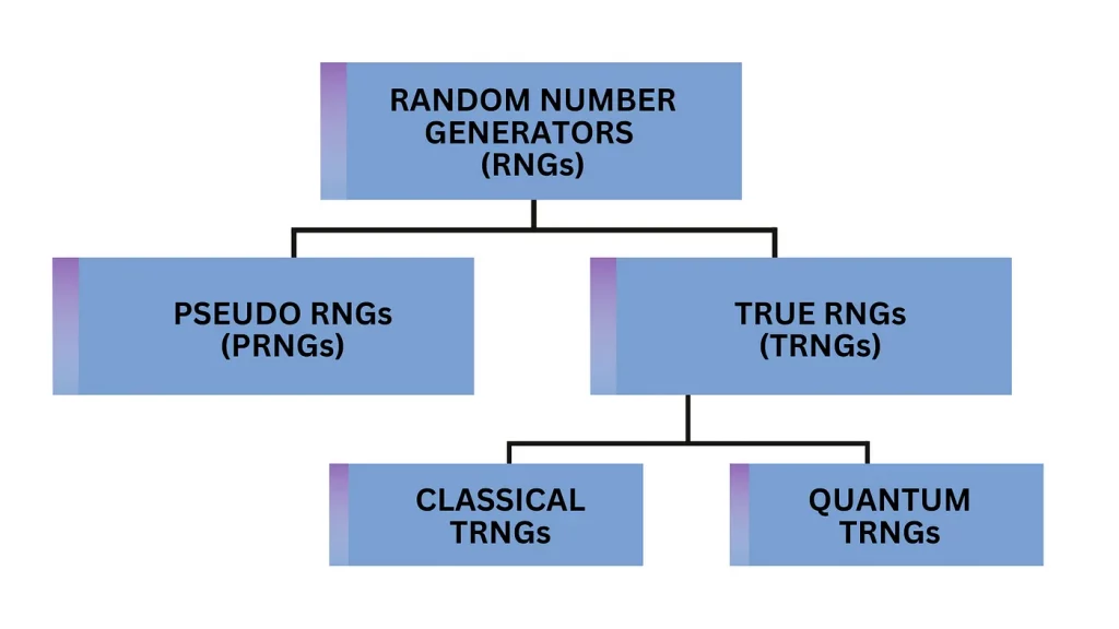
We’ve already talked about two Random-Number Generators (RNGs), the coin flip and the radioactive cesium, both of which are examples of true RNGs. That is, they rely on unpredictable physical processes (or, rather, not-easily-predictable) to make their lists of 0s and 1s. But there are many kinds of RNGs, which you can see in Fig. 1
Fig. 1: Various classes of random number generators discussed in this article.
The one programmers are probably most familiar with is pseudo-RNGs. Here, you give a random seed number to a mathematical algorithm, which uses that number to deterministically generate a longer list of numbers that look random. While this is a convenient way to generate random numbers, there is a big caveat: if someone ever gained access to your seed numbers, past or present, they could replicate all of your numbers for themselves!
Then you have true RNGs, of which there are two main kinds: classical and quantum. These are based on unpredictable physical processes. A simple example of a classical true RNG is the coin flip, but there are many more complex methods that are used in modern electronics, for example measuring thermal noise from a resistor. The Achille’s heel of classical true RNGs is that while the details of the generating process may be unknown, they are still in principle knowable. What are the implications of this? Well, if a bad guy wants to know your random numbers, they can always build a better model of your classical system for better predictions. Your classical RNG must therefore necessarily be complex.
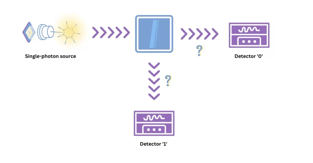
Quantum true RNGs can do better. Rather than watching our stolen cesium beta-decay, we’ll take an example from quantum optics (see Fig. 2). Here, a train of single photons is shone onto a semi-transparent mirror, which has two outputs. Because quantum mechanics is inherently unpredictable, the single photon will randomly take one of these two paths, after which it can be measured by one of two detectors, which correspond to 0 or 1. This is good at first sight, but be careful: in an ideal world, where all of the photons really are single, the beam splitter doesn’t absorb any photons, and the detectors don’t have any noise or loss, then we really do get independent and identically distributed random numbers. But this is not an ideal world, and so we call this kind of quantum RNG device-dependent because we must trust the physical engineering of the RNG. However, quantum RNGs are still a step in the right direction because we do not have to complexify them like in the classical case.
Fig. 2: An example from quantum optics of true random number generation. Single photons are shone onto a semi-transparent mirror, and they will randomly go to detector 0 or 1.
Now, we wouldn’t have given the previous example a fancy name like device-dependent quantum true random number generator if there wasn’t also such a thing as device-independent quantum RNGs — the holy grail of RNGs. The latter devices can generate and validate their own random numbers: they are certifiably random, independent of the underlying hardware. But how can we make such a thing? We use entanglement.
Essentially, if Alice and Bob share two entangled particles, and Alice measures her particle, then the state of Bob’s particle is instantly changed according to Alice’s measurement, no matter how far apart they are. This is a fundamentally quantum effect which cannot be described classically. But we have to be careful that Alice and Bob aren’t cheating. If Alice and Bob are physically too close, then we don’t know if they’re secretly sharing information to coordinate their measurements. When they’re sufficiently separated, we call this nonlocality.
So, if Alice and Bob create a pair of entangled particles, then randomly choose how to measure them, the outcomes of their measurements are quantum-certified random so long as satisfy the nonlocality condition (and a couple of other secondary conditions which are beyond the scope of this article; see Quandela’s recent publication on quantum RNGs).
Because of nonlocality, these kinds of random-number experiments tend to be big so that the measurements are far, far apart. In a world which is both obsessed with small, scalable devices and also maximum security, how can one reconcile this paradox? This is exactly the problem that researchers at Quandela have solved.
Part 3: Quandela’s contributions
They ask:
‘How can we certify randomness generation in a device-independent way with a practical small-scale device, where [Alice and Bob could cheat thanks to communication] between the physical components of the device?’
Put another way, when you have a small device that might normally allow Alice and Bob to cheat by communicating information before the other one measures their particle, can you account for this local communication somehow to still generate certified random numbers? Quandela’s protocol measures the amount of information that an eavesdropper could potentially use to fake violation of locality, and then sets a bound on how well the device should perform if it is to still produce certified random numbers. The device also periodically tests itself to validate these numbers.
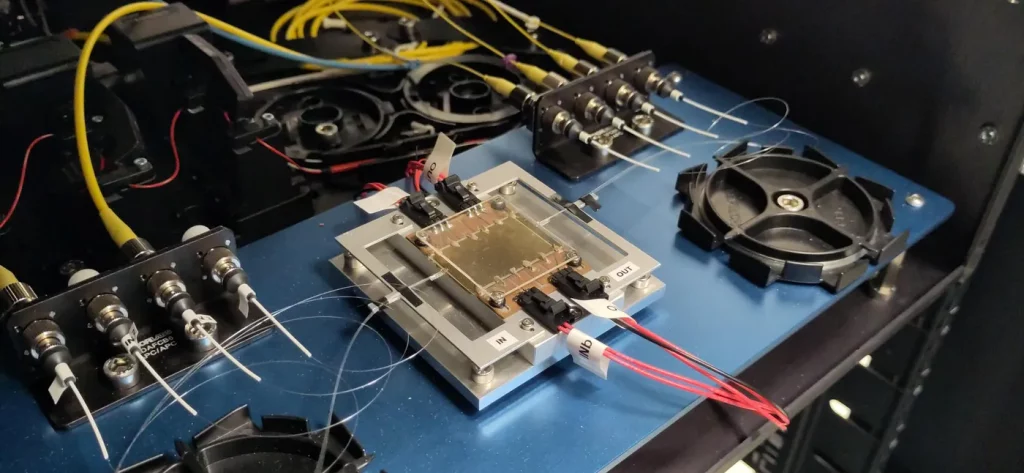
And not only has Quandela derived the theory, but they’ve also demonstrated it experimentally on a two-qubit photonic chip using Quandela’s patented single-photon quantum dot source, show in Fig. 3.
Fig. 3: Quandela’s two-qubit random number generator.
If this all sounds like a big deal, that’s because it is — the technical details are all found in the recent publication, with a patent on its way!
This achievement represents a major step towards building real-world, useable quantum-certified random number generators, one more tool in Quandela’s arsenal of quantum technologies.
If you are interested to find out more about our technology, our solutions, or job opportunities, visit quandela.com.
Quantum computing is at the forefront of technology, with the potential to transform how we process information. This emerging field leverages quantum phenomena such as quantum superposition and entanglement to accomplish computational tasks at unprecedented speeds. Among the different strategies for achieving quantum computing, photonic quantum computing is a particularly bright star.
Photonic quantum computing uses light particles — photons — as the carrier quantum information. This approach has many benefits ; photons are stable, they have modest cooling requirements and they are scalable.
One method for encoding information in photonic quantum computing is ‘dual-rail encoding’. In dual rail encoding a pair of tracks form a qubit where the logical (1) is encoded in the photon traveling in the lower rail and the logical(0) is encoded in the photon traveling in the upper rail. This reliable encoding method is widely used in the photonic world. More details can be found here.
In a significant leap forward in this field, we at Quandela have developed Ascella[1], a general-purpose single-photon-based quantum computing platform. Ascella is a quantum computer that uses a highly efficient quantum dot single photon source, which functions much like a miniature box that produces single photons on-demand which then go into its universal interferometer to perform the computation and subsequently are detected at the output for processing. More details about single photon sources here.
To compensate for hardware errors, Ascella uses a machine-learned transpilation process. Transpilation is the process of rewriting a given input circuit to match the topology of a specific quantum device. Additionally, it features a full software stack that enables remote control of the device, opening up opportunities for a range of computational tasks through logic gates or direct photonic operations.
At Quandela we have successfully demonstrated high-fidelity one-, two-, and three-qubit gates, implemented a complex quantum algorithm to calculate the ground-state energy of the hydrogen molecule and even developed a photon-based quantum neural network. Notably, Ascella achieved the generation of a unique type of quantum entanglement involving three photons — heralded 3-photon entanglement. This achievement is a critical milestone toward ‘measurement-based quantum computing’ a promising pathway to scale up quantum computers (*).
(*) Measurement-Based Quantum Computing (MBQC) is a form of quantum computing where computation is performed through a sequence of single-qubit measurements on a pre-established, highly entangled state known as a cluster state. In this model, the process and outcome of computation are determined by the choice and order of measurements
Diving Into Ascella’s Architecture SECTION 1
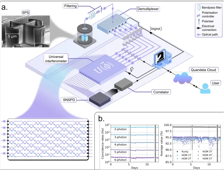
At its core, Ascella is a unique piece of technology that uses light to perform complex calculations. Its hardware is made up of several key components. Firstly, there is the single-photon source which produces the photons on demand. This source emits photons into a fiber which then sends the photons on their journey through the system. The system contains a device called a demultiplexer, which is responsible for splitting the stream of photons into separate streams. So it feeds the chip 6 photons that arrive at the same time. Secondly there is the unitary matrix in the universal interferometer which determines the evolution of the photons and finally detectors (SNSPD) at the outputs.
FIG. 1: Architecture, performance and stability of Ascella.
1.1 Peering into Ascella’s Operational Mechanism
Quantum interference is what enables Ascella’s operations. At the heart of the system is an integrated circuit, containing a multitude of voltage-controlled phase shifters and beamsplitters. This circuit can be programmed to perform a variety of tasks, transforming the photons’ states as they move through the circuit. These photons are then detected and recorded, creating the output data from Ascella.
1.2 Stability and Performance
Just like a well-oiled machine, Ascella needs to perform consistently over time. To ensure this, key performance metrics are monitored and the system undergoes automatic hourly optimizations. This commitment to performance maintenance allows Ascella to remain stable and high performing for weeks on end, an essential quality for any computing platform and especially for the demanding realm of quantum computing.
1.3 Ascella’s User Interface
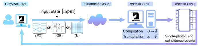
Ease of use is another important aspect of Ascella’s design. Users can interact with Ascella remotely using the open-source Perceval framework. This allows users to send tasks, such as specifying a certain pattern for the photonic circuit or requesting a specific transformation on an input state, which could contain anywhere from one to six photons. The results are then sent back to the user.
FIG. 2: From Perceval User to Ascella QPU. PC = Photonic circuit, GB = Gate based, U= Unitary, ɸ= Phase shifts, V= Voltages
Ascella represents an exciting stride towards scalable quantum computing. It operates a record-breaking number of single photons on a chip and its robust capabilities combined with a user-friendly interface making it a promising player in the noisy intermediate-scale quantum (NISQ) computing era.
Understanding the behavior of molecules is critical in fields like chemistry and medicine. However, simulating molecular behavior can be incredibly complex for classical computers, especially when it comes to quantum phenomena. Ascella, Quandela’s photonic quantum computer takes advantage of the Variational Quantum Eigensolver (VQE), a tool for quantum chemistry.
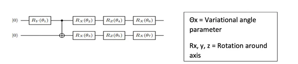
The VQE is a hybrid quantum-classical algorithm that can estimate the ground state energy of a molecule, providing insight into its lowest energy configuration. This ground state knowledge is crucial as it can help predict how a molecule will react in a chemical reaction, which in turn, can lead to new drug developments or more efficient materials for energy production. In our case the VQE algorithm was used on a H2 molecule with the following ansatz.
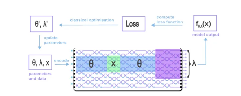
This is where the “variational” part of VQE comes in: it iteratively varies the parameters of the wavefunction to find the one that gives the lowest energy. This is done in a feedback loop, where the quantum computer calculates the expectation value, then a classical computer updates the parameters and directs the quantum system to recalculate based on these new parameters.
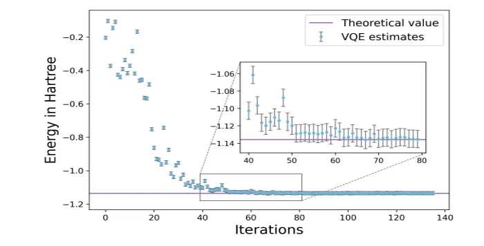
FIG. 4: Energy (Hartrees) vs iterations for VQE run on Ascella. We observe a convergence to the true theoretical value.
In practice, Ascella’s VQE consistently converges to the theoretical energy eigenvalue within 50 to 100 iterations, regardless of the initial random parameters or bond length. In tests, the algorithm achieved chemical accuracy — an error of only ±0.0016 Hartree, a unit of energy in the atomic scale — with a success probability of 93%. These significant improvements can be attributed to the high-quality single-photon sources and advanced control of the photonic chip.
Ascella’s Quantum Neural network/Variational quantum algorithm for classification: SECTION 3
Quandela has successfully constructed and trained a quantum neural network (QNN) for a supervised learning classification task using our advanced quantum computing platform, Ascella. In designing our approach, we utilized a variational quantum algorithm (VQA) for constructing the QNN. Similar to classical neural networks, where interconnected neurons are represented by numerical weights and biases, a QNN consists of qubits manipulated by quantum gates. The parameters of these quantum gates, analogous to the weights and biases in classical networks, are adjusted during the learning process to minimise some cost function.
The VQA represents a hybrid quantum-classical strategy, where the quantum device prepares a quantum state dependent on a set of parameters, and the classical device estimates a value for that state.
FIG. 5: The trainable blocks parameterised by θ are depicted in blue. The data encoding block is in green. The model is computed by assigning λ parameters to the outputs at the detectors.
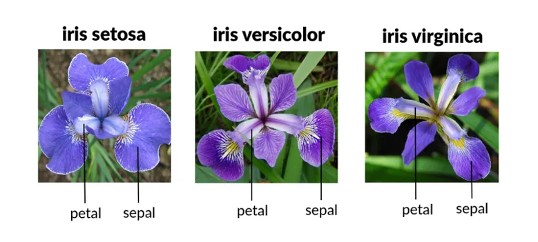
We developed our quantum algorithm with a photonic ansatz. This ansatz was designed directly on Ascella by using beam splitters and phase shifters. We then applied this methodology to the Iris dataset, which contains measurements such as petal and sepal sizes from different species of Iris flowers. The task was to predict the Iris species based on these measurements.
FIG. 6: Iris dataset samples
This experiment constitutes an application of a variational quantum classifier with single photons, a notable achievement. This process yielded an accuracy of 92% on the training set and an even higher 95% on the test set after about 15 iterations.
In summary, our represents an important step in quantum machine learning. By successfully training a QNN on a classic machine learning problem, we have demonstrated the potential for quantum computers to process complex data efficiently. This successful application of a variational quantum classifier with single photons heralds exciting possibilities for the future of quantum computing and machine learning.
A quantum over classical computational task: Boson sampling SECTION 4
In a step forward for our quantum computing approach, we have conducted an experiment in Boson Sampling with six single photons.
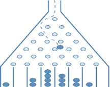
Let’s explain what this means, starting with Boson Sampling. Think of this as trying to predict how a bunch of photons (particles of light) will distribute themselves after passing through a complex network of mirrors and splitters. The classical version, a Galton board might help visualize this with a ball moving between pegs and creating like such.
FIG. 7 : Galton board
However, the real quantum task is much more complex. Unlike balls on a Galton board, photons interfere with each other in a quantum mechanical way, leading to a highly complex probability distribution of the output states. Simulating this process with classical computers is incredibly difficult, but a quantum computer, mimicking the physical processes involved, can solve this problem naturally.
Our experiment involves performing Boson Sampling for a record number of six photons with a fully reconfigurable interferometer. An interferometer is a device used to split and recombine beams of light, creating an interference pattern that can be measured.
In the experiment, we measured the occurrences of photon coincidences (when multiple photons are detected at the same time) for up to six photons. We then compared the observed distribution of photon outputs to the ideal distribution predicted by our model.
This accomplishment is a significant stride and step forward for quantum computing, we have conducted an experiment in Boson Sampling with six single photons with high fidelity, demonstrating this quantum-over-classical computational task.
We are pushing the boundaries of our quantum computing capabilities. As of now, we’ve achieved an operation speed that is quite impressive. And we believe this speed can be further improved by optimizing each component of our system.
One such component is the single-photon source, which essentially generates the tiny particles of light, or photons, that carry information in this system. Currently, it’s operating at about 55% efficiency[i]. With advancements in technology, we believe that we can increase this efficiency by up to 96%. This means the platform will generate almost twice as many usable photons as it currently does, a significant increase in data processing potential.
Additionally, we have plans to increase the size of the interferometer on the chip we’re using. This mean the chip can process more information simultaneously, which means that we can run tests on larger molecules than H2 and more sophisticated algorithms in general.
An essential part of this exploration involves GHZ states. These are specific entangled configurations in a quantum system involving three or more particles. Creating and controlling these GHZ states is a significant milestone in quantum computing. It represents our growing ability to manipulate complex quantum entanglements involving multiple particles, a crucial aspect of measurement-based quantum computing (MBQC). Even more impressively, on the Ascella project we managed to generate these GHZ states predictably or in a “heralded” way. That means we could not only anticipate the creation of these states but also confirm when they occurred.
The successful implementation of these heralded entanglement schemes opens the door to fault-tolerant quantum computing. It’s an exciting time for quantum computing, and we’re thrilled to be at the forefront with Ascella!
References:
1. Nicolas Maring, Andreas Fyrillas, Mathias Pont, Edouard Ivanov, Petr Stepanov et al
[i] A single photon source that operates at 100% efficiency would emit a single photon each time it is triggered. At 55% efficiency it would emit a single photon each time it is triggered 55% of the time.
Quantum mechanics is intrinsically random. When a quantum state undergoes an evolution through a quantum process, the output state is a well-defined mathematical object, but we can only access it through measurements. Each measurement produces an output that belongs to a probability distribution that follows the Born rule. This could be seen as a bottleneck for a quantum developer compared to classical computation. But when quantum information is used cleverly, we can encode the results of our problem in a few measurement outcomes enabling solving challenging problems for classical computing (see Shor algorithm example for instance here) .
What do people call a shot in the context of quantum computing?
One “shot” represents one execution of a quantum circuit. Given the probabilistic nature of the system, conducting multiple iterations of the system (obtaining many shots) is necessary to gather data for statistical analysis of the algorithm’s operation. The concept of “shots” is universally embraced by most quantum providers. But the precise implementation of “shots” and their management will vary among different frameworks as it depends on the specific characteristics of the hardware system.
How do we define shots at Quandela?
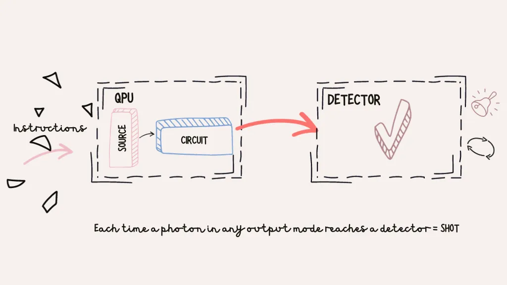
Our computing architecture works with linear optics. We send single photons in a quantum circuit composed of tunable linear optical elements which results in an operation optical elements forming the quantum circuit performing the processing action on states of photons (input source) acting as a qubit in the Fock space (for an explanation of the Fock space see here). A photon-coincidence event — detection of at least 1 photon at the output — Detection of 1 or multiple photons by the detectors at the output defines a single execution of a quantum experiment.
Each time a photon in any output mode reaches a detector = SHOT
Our QPU sends single photons at a periodic rate into the chip implementing the circuit designed by the user. While these photons may undergo absorption at various points within the hardware. Nevertheless, whenever at least one photon is detected at the optical chip’s output (termed as a photon-coincidence event), it marks the end of a single execution and the measured output constitutes a data samplewe consider that the quantum circuit has been executed. Our shot count is thus defined as the number of photon-coincidence event during the computation.
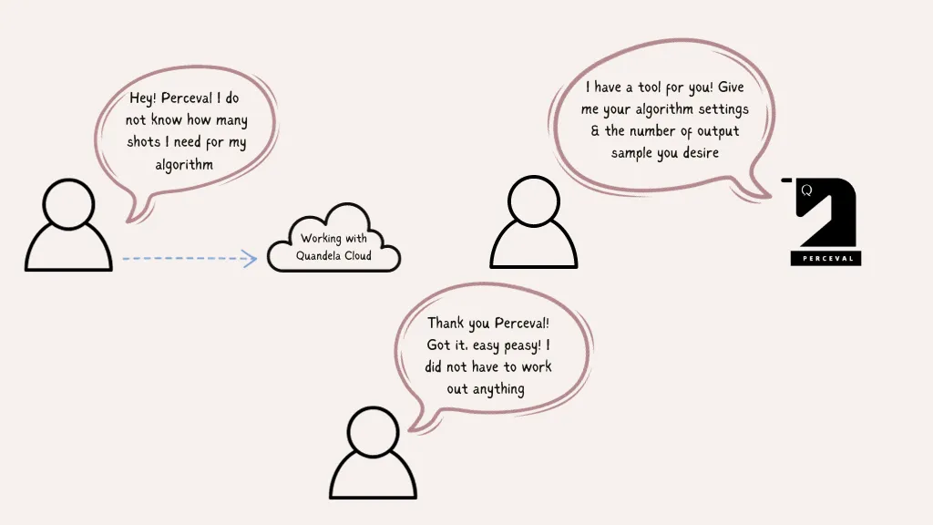
Perceval is able to provide the number of shots needed
A user may not necessarily want to sample single photon detections; they may specifically desire samples with a certain number “N” (>1) of photon coincidences and request these as the output. In such cases, the system may need to be run with a number of shots exceeding the requested number of samples, as multiple photon coincidences are anticipated. Recognizing this user preference, we have incorporated a tool in Perceval to calculate estimate the necessary number of shots based on the user’s desired sample count. This tool conducts the estimation by considering the unitary of the implemented circuit, the input state, and the performance characteristics of the device.
How Shots will Revolutionise our User’s Experience?
Access to Quantum State Distribution: In the light of the definition that characterises “Shots” as the output detected during each circuit execution, they offer direct access to the probability distribution of a quantum state.
Predictable output rate: In a photonic system characterised by instantaneous gate applications and a complex input state preparation timing (see detail on demultiplexing here), the time capture of shots clearly indicating the end of a single execution is exhibiting variability attributed to this input state time sequence, the actual configured circuit, and system transmittance factor. Working with shots guarantee a predictable output rate independent of these fluctuations.
Simplified User Interactions: The incorporation of shots not only seeks to standardize user interactions with running algorithms on our Quantum Processing Unit (QPU) through our cloud services but also provides them with a more standardized parameter for understanding their resource needs. This enhancement contributes to a clearer and more consistent measure.
Predictability for Time and Cost: -Shots, being highly predictable, offer the most reliable means to estimate the time and cost of running an algorithm. -This stability in parameter counting results in fixed pricing, ensuring fairness to users and independence from the variability of the performance of the physical QPU device.
If you are interested to find out more about our technology, our solutions or job opportunities visit quandela.com
One of my fondest childhood memories is enjoying the sweet, delicious taste of a large-scale fault tolerant quantum computer. In this article, we’re going to explain how you can bake your own scrumptious quantum processor from scratch. Whether you’re trying to impress a first date, cater for friends, or entrench a technological advantage against your geopolitical rivals, quantum computers are the perfect treat for any occasion.
Difficulty: Extreme
Cooking time: 5–7 years of R&D
In our last article, we answered the question “What is a Quantum Computer?”. As a quick reminder: a quantum computer is a device that uses the principles of quantum mechanics to perform certain calculations much faster than a regular computer.
One of the most common recipes for baking a quantum computer was created by quantum chef/scientist David DiVincenzo. His family recipe lists 5 main ingredients (we’re dropping the cake analogy from here on for clarity):
1. A scalable physical system of qubits
A classical computer uses binary bits with a value of either 0 or 1 to represent information. This is represented physically as tiny switches called transistors inside the computer that are either on or off. Quantum computers often represent information as qubits, which can be in the state |0>, |1>, or a superposition of both states. For a proper explanation of how this works, check out our previous article.
Many different physical systems have been used to generate qubits, including superconductors, ion traps, and photons. It’s important to highlight that the system of qubits must be scalable i.e. we can create larger and larger systems of connected qubits to run larger calculations. The quantum computers available in labs today don’t have enough processing power to tackle real world problems. If a system of qubits can’t be scaled up, we won’t be able to use it to create useful quantum computers.
2. The ability to initialise the qubits to a simple reference state
Imagine trying to do maths on a calculator without being able to erase the answer to the previous calculation, or even check what it was; the errors would be enormous. Initialising states is necessary for both classical and quantum computers, but for quantum computers it’s much more difficult.
The initialisation process varies depending on the qubit’s physical system. Let’s examine the case of photonic qubits discussed in our previous article. In this system, a photon can be in one of two optical fibres. The system is in the state |0> or |1> depending on which fibre the photon is in. A simple reference state for this system would be |0000>, which means that 4 qubits have a photon in the fibre corresponding to their |0> state. To initialise this kind of photonic qubit you need to be able to emit single photons, on demand, into specific optical fibres.
This sounds easy, until you consider how small photons are. A normal LED lightbulb releases quintillions of photons every second. Releasing just one of them (and controlling it) is extremely difficult. Quandela was founded on technology which tackles this very problem, by fabricating semi-conductor quantum dots that act as controllable single-photon sources. You can learn more about our technology in this article.
3. Decoherence times that are much longer than the gate operation times
Most types of qubits are extremely delicate, and they tend to lose their quantum properties (such as superposition, entanglement, and interference) soon after they are initialised through a process called decoherence. Decohering qubits ruin quantum computations, which rely on such quantum properties to deliver all the nice speedups and advantages that they have when compared to ordinary classical computers. So the operations we use to manipulate quantum states (performed by quantum gates) must be fast relative to the lifespan of the qubit, or some of them may decohere before the calculation is finished. In our food analogy, you can’t make a meal using ingredients that will expire before you’re finished cooking them.
4. A universal set of quantum gates
Quantum gates are the quantum versions of the logic gates used in classical computers. They affect the probability of getting a particular answer when the qubits they act on are measured (see previous article for details). Some gates act on one qubit at a time, while others act on two or more. A universal set of gates is a group of gates that you can combine to form any other gate. If you have a universal set of gates, you can perform any quantum operation on your qubits (ignoring gate errors, decoherence, and noise, which we will discuss further in a future article).
5. A qubit-specific measurement capability
There wouldn’t be much point in performing calculations on a quantum computer if you couldn’t record the results. A measurement is said to be qubit-specific if you can pick out a particular qubit and detect what state it is in: usually |0> or |1>. This gives you the result of your quantum calculation as a string of 0s and 1s, which could eventually be fed into a classical computer to design life-saving medicine or decrypt your internet search history.
Quantum Communication
DiVincenzo outlined two additional criteria to allow a device to engage in quantum communication, which is the transfer of quantum information between processors separated by a large distance. These criteria are:
The ability to convert between stationary qubits (used for calculations) and flying qubits (that can move long distances).
The ability to faithfully transmit flying qubits between specified locations.
Quantum communication allows us to connect quantum computers together and combine their processing power to solve problems. Photons are the best option, and in fact probably the only sensible option, for implementing flying qubits, given that they travel at the speed of light, don’t suffer from decoherence over time (although optical components still add noise), and can be directed through optical fibres.
What now?
The DiVincenzo criteria have had an enormous impact on the field of quantum computing research over the past two decades. Unfortunately, they may also restrict our understanding what a quantum computer can be. We will explore this further in the next article of this series, which explains why the number of qubits in a quantum computer doesn’t necessarily measure how advanced it is.
Having read this and the previous article, you should now have a basic understanding of what quantum computers are, how they work, and what it takes to cook one up from scratch. Follow Quandela on Medium to learn more about quantum computing from one of the most advanced companies in the field.
Disclaimer: Cooking time may vary. Quantum computers are hardware devices which may be composed of high energy lasers, powerful magnets, and silicon chips at temperatures close to absolute zero. They are not food. Please do not attempt to eat a quantum computer. Quandela does not accept any liability from readers attempting to consume the components of a quantum computer.
Quantum computing has the potential to be one of the defining technologies of the 21st century, with practical applications that could completely transform modern society. Despite its enormous significance, most people have absolutely no idea what quantum computing is.
In this article, we’re going to explain what quantum computers are and give a brief introduction to how they work. You don’t need a background in science to follow along, just a few minutes of spare time and a desire to learn.
What’s the definition?
A quantum computer is a device that uses the principles of quantum mechanics to perform certain calculations much faster than a regular computer. When we say faster, we don’t mean that scientists will spend less time waiting around for their results. A future large-scale quantum computer could solve problems that would take millions of years on today’s best supercomputers (1,2).
These problems aren’t just abstract maths puzzles, they’re real-world challenges that will have a massive impact on people’s lives. Quantum simulations of chemical reactions would enable the discovery of life-saving medicines, advanced materials, and sustainable manufacturing processes (3–5). Quantum algorithms could lead to breakthroughs in artificial intelligence, while quantum cryptography could provide unbreakable data encryption secured by the laws of physics[1] (6,7). The significance of these applications has led to a lot of hype around quantum computing, eagerly fed by companies in the industry looking to secure customers and raise funding. To cut through this hype and understand the underlying technology, we need to look at some fundamental physics.
What is Quantum Mechanics?
The basis of quantum computing is quantum mechanics, which is a scientific theory that describes the behaviour of the basic building blocks of our universe, like atoms, electrons, and photons[2]. Let’s quickly define two important terms: a “quantum system”is something whose behaviour can be explained through quantum mechanics, and a “quantum state” is the mathematical description of a quantum system.
The key principles of quantum mechanics that you’ll need to understand quantum computing are entanglement, interference, and superposition:
Entanglement: When a group of particles are entangled, measuring one of them instantly causes a change[3] in the others, even if they are vast distances apart. In technical terms, the quantum states of entangled particles can’t be described independently of one another.
Entanglement doesn’t exist in our large-scale everyday world, so it can be hard to wrap your head around it. As an example, imagine that we had a pair of entangled quantum coins, which each exist as a combination of heads and tails at the same time until we measure them[4] (I never said it would be a good example). If I flipped one of the coins and it landed on heads, then I could know with 100% certainty that yours would be tails before you’d flipped it. The instant its entangled partner was measured, your coin was in the state tails, instead of the combination of heads and tails it was the moment before.
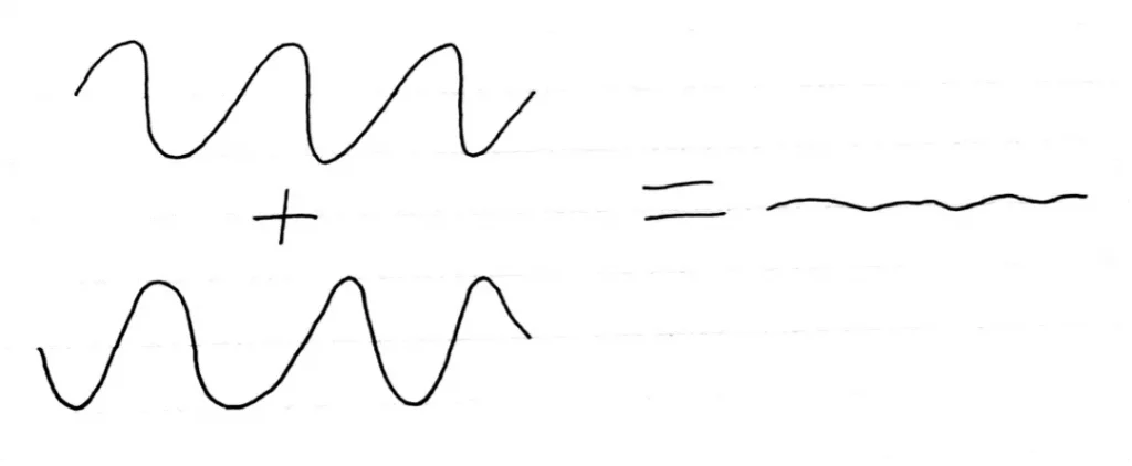
Interference: Interference is a phenomenon where overlapping waves combine or cancel out. It’s how noise-cancelling headphones work: they emit sound waves that interfere destructively with background noise. A simple diagram of destructive interference is shown below:
Waves canceling out through interference
Quantum particles can act like waves, so they experience quantum interference. The maths describing quantum interference is a bit different to regular interference, but the general idea is the same.
Superposition: A quantum state can be described mathematically as the sum of other quantum states. This is another similarity between quantum states and waves, which can be described as the sum of other waves. The quantum coin existing as a combination of heads and tails in our entanglement example was in a superposition of heads and tails.
Quantum mechanics is one of the most stunningly accurate scientific theories in history, but an engineer would never use it to design a car or a bridge. Instead, they’d use the rules from a less precise group of theories known as classical physics.
Classical physics is a set of approximations and simplified rules used to describe the stuff we interact with every day (heat, sound, motion, gravity, etc.). These are the laws of physics you probably studied in school. When many quantum objects interact, it becomes easier to describe their collective behaviour using classical physics rather than quantum mechanics. A football is made of atoms, but you don’t need quantum physics to predict what will happen if you kick it. “Classical” in this context refers to the non-quantum, large-scale, everyday world of footballs and kicking that we live in.
To explain how quantum computers use entanglement, interference and superposition to perform calculations, we’re going to examine qubits: the fundamental components of (most[5]) quantum computers.
What is a Qubit?
A classical computer like the device you’re reading this on uses bits to represent information. A bit can have a value of 0 or 1, like a switch that is either on or off. Modern computers are made of billions of these tiny switches, allowing them to perform complex tasks such as delivering your daily meme supply. For instance, the word “Hi” is stored in a computer (using ASCII binary code) as 1001000 1101001. As well as storing information, computers perform calculations using bits: 2 + 2 = 4 is represented in binary as 10 + 10 = 100.
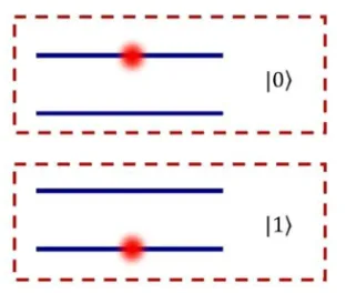
The quantum version of a bit is called a qubit. Physically, a qubit is just a two-level quantum system. One example of a qubit is a photon that can be sent down either of two optical fibres. An optical fibre is a wire made of flexible glass or plastic that reflects photons internally. It can be used to transport light like copper wire carries electricity.
If the photon is in the first of the two fibres, then the qubit is in the state |0>. If the photon is in the second fibre, then the qubit is in the state |1>. When you measure the state of this qubit by detecting where the photon is, you’ll get a classical 0 or 1. This is shown in the diagram below:
Travel path photonic qubits
Quick note: |x> is how we write a quantum state in Dirac notation, which is a convention that makes quantum physics calculations easier.
One of the weird features of quantum mechanics is that a single photon can be sent down both fibres at the same time, as a superposition of the two states. Measuring the photon causes the superposition to collapse, and the photon will be found in one fibre or the other. Qubits existing in a superposition is one of the key differences between quantum and classical computing, which will be discussed further in the next article of this series.
How do we use this for calculations?
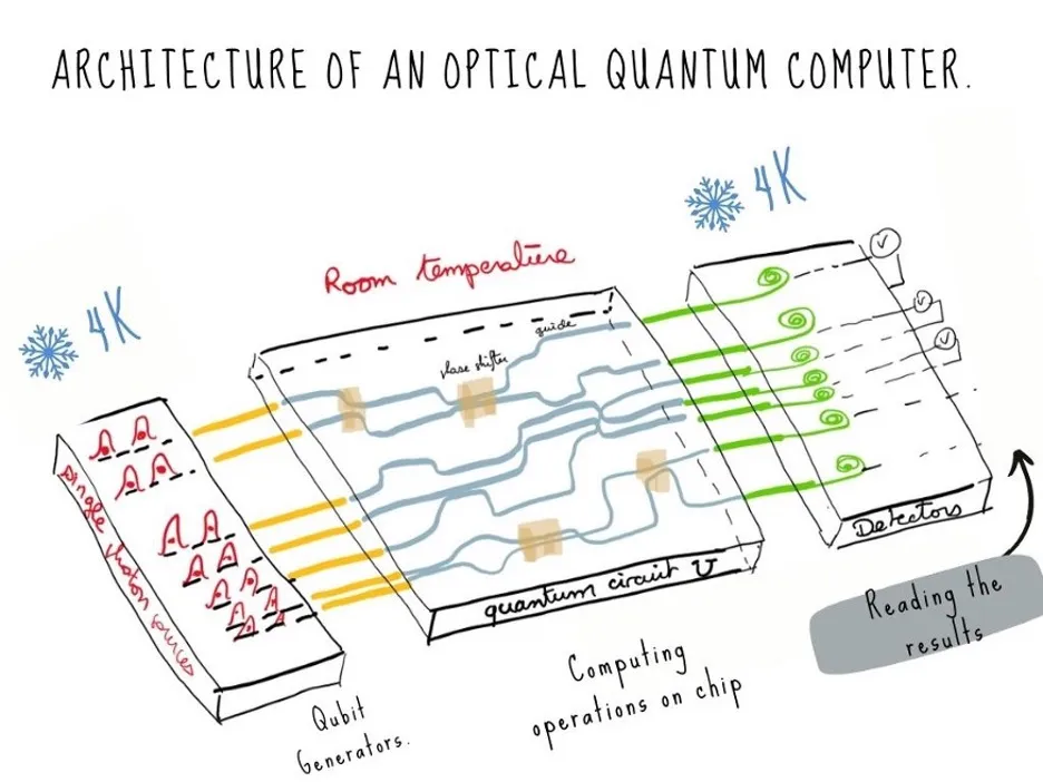
A qubit-based quantum computer is generally composed of three stages:
1. Initialisation: The qubits are given a known value when the calculation starts, such as every qubit being in the state.
2. Manipulation: A quantum circuit uses interference and entanglement to apply mathematical operations to the qubits.
3. Measurement: The quantum states of the qubits are measured to read the results of the calculation.
An example of this structure can be seen in the following diagram of a photonic quantum computer:
Architecture of an optical quantum computer
At the end of a calculation, the qubits in a quantum computer exist in a superposition of all the possible outcomes. When you measure the qubits, you collapse this superposition, and get one of the possible outcomes at random as your answer. Quantum algorithms can be designed so that the quantum states in the superposition corresponding to the wrong answers interfere destructively and cancel out, leaving behind only the right answers. Entanglement is used to connect qubit superpositions together to perform useful calculations.
By running the circuit and measuring the qubits hundreds or thousands of times, we can build a graph of how likely each of the possible outcomes are. This graph (a probability distribution) is the final result of our quantum calculation.
The process of manipulating probabilities with superposition, interference, and entanglement is fundamentally different to how normal computers operate. That is why quantum computers can do certain tasks so quickly: they’re not better than classical computers in general, they just work differently. Quantum computers are much better suited to mundane supercomputer-style tasks like designing medicines than crucial everyday tasks like posting memes, so they are expected to co-exist with classical computers rather than replacing them entirely. Many of the most famous quantum algorithms actually use a combination of quantum and classical techniques to solve problems[6].
What’s next?
Hopefully this explanation has given you a basic understanding of what a quantum computer is. In the next article in this series, we’re going to examine how a quantum computer works in more detail, hopefully without getting lost in technical jargon.
If you are interested to find out more about our technology, our solutions or job opportunities visit quandela.com
Footnotes:
1. Optical quantum communications can provide data protection through security protocols such as BB84, while quantum computers will be able to factor large numbers using Shor’s Algorithm and break modern RSA encryption. There are, however, non-quantum encryption techniques that are immune to Shor’s algorithm.
2. Atoms are not elementary particles like quarks and gluons, but they are still small enough to be described with quantum mechanics. Quantum mechanics is also needed to explain certain behaviours of some large-scale objects like black holes and neutron stars.
3. Entanglement is a slippery subject. Technically change occurs in the quantum states of the other particles; i.e. their mathematical descriptions. An important side point is that the change is not directly observable, except through clever strategies which involve comparisons of observations on each particle. If the changes were directly observable it would provide a means of instantaneous (faster-than-light) communication across great distances — something that’s already disallowed by relativity, one of our other great theories of physics.
4. Maybe you could begin to wonder at this point whether this combination of heads or tails is really all that strange… After all I could perform a coin flip, close my fist around it to catch it, and until I open it again I won’t know if it’s a head or a tail. That’s a kind of combination of heads and tails too, right? Well, yes, but this is where everyday and quantum coins begin to differ. The everyday coin really is just one or the other, and all that’s really happening is that I’m ignorant and don’t have the information about which one it is yet. On the other hand, a quantum coin can really be in a superposition of both heads and tails. And we can know that it’s in a genuine superposition by doing clever experiments that look for interference effects.
5. Photonic quantum computers can demonstrate quantum advantage using a technique called Boson Sampling without encoding information as qubits. We will explain this in detail in a future article.
6. Some examples of quantum-classical algorithms include Shor’s Algorithm (8), VQE (9), and QAOA (10).
References
1. Arute F, Arya K, Babbush R, Bacon D, Bardin JC, Barends R, et al. Quantum supremacy using a programmable superconducting processor. Nature. 2019 Oct;574(7779):505–10.
2. Madsen LS, Laudenbach F, Askarani MFalamarzi, Rortais F, Vincent T, Bulmer JFF, et al. Quantum computational advantage with a programmable photonic processor. Nature. 2022 Jun 2;606(7912):75–81.
3. Kirsopp JJM, Di Paola C, Manrique DZ, Krompiec M, Greene-Diniz G, Guba W, et al. Quantum Computational Quantification of Protein-Ligand Interactions [Internet]. arXiv; 2021 [cited 2022 Jul 19]. Available from: http://arxiv.org/abs/2110.08163
4. Clinton L, Cubitt T, Flynn B, Gambetta FM, Klassen J, Montanaro A, et al. Towards near-term quantum simulation of materials [Internet]. arXiv; 2022 [cited 2022 Jun 24]. Available from: http://arxiv.org/abs/2205.15256
5. Greene-Diniz G, Manrique DZ, Sennane W, Magnin Y, Shishenina E, Cordier P, et al. Modelling Carbon Capture on Metal-Organic Frameworks with Quantum Computing [Internet]. arXiv; 2022 [cited 2022 May 17]. Available from: http://arxiv.org/abs/2203.15546
6. Havlicek V, Córcoles AD, Temme K, Harrow AW, Kandala A, Chow JM, et al. Supervised learning with quantum enhanced feature spaces. Nature. 2019 Mar;567(7747):209–12.
7. Bennett CH, Brassard G. Quantum cryptography: Public key distribution and coin tossing. Theor Comput Sci. 1984 Dec;560:7–11.
8. Shor PW. Polynomial-Time Algorithms for Prime Factorization and Discrete Logarithms on a Quantum Computer. SIAM J Comput. 1997 Oct;26(5):1484–509.
9. Peruzzo A, McClean J, Shadbolt P, Yung MH, Zhou XQ, Love PJ, et al. A variational eigenvalue solver on a quantum processor. Nat Commun. 2014 Sep;5(1):4213.
10. Farhi E, Goldstone J, Gutmann S. A Quantum Approximate Optimization Algorithm [Internet]. arXiv; 2014 [cited 2022 Jul 20]. Available from: http://arxiv.org/abs/1411.4028