Article by Sebastien Boissier

Deterministic sources by Quandela

This is part three of our series on single-photon sources. Building on our previous posts, we finally have the necessary context to discuss Quandela’s core technology and how it will accelerate the development of quantum-photonic technologies towards useful applications.

Atoms

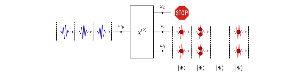
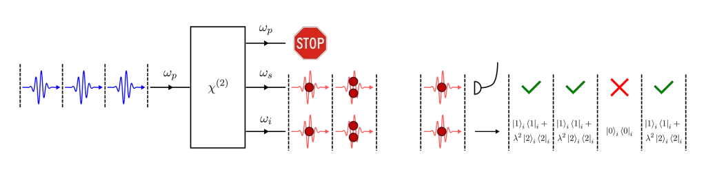
Even though heralded photon-pair sources are a well-known technology, it does seem to be a bit of a work-around to achieve our primary goal of generating pure single-photons. The fact that they are inherently spontaneous is an issue, and we would prefer to avoid multiplexing which is resource hungry. OK then, is there another approach?

Atom-light interaction

An elegant idea comes from our knowledge of how light interacts with single quantum objects such as atoms. In this context, what we really mean by a “single quantum object” are the quantised energy levels of a bound charge particle. In a hydrogen atom for example, the electron is trapped orbiting around the much-heavier proton and it can only exist in one (or a superposition of) discrete quantum states.

When we shine a laser on an atom, we can drive transitions between two states. For example, the electron can be promoted from its ground state to a higher-energy excited state. In general, there are certain constraints that the pair of states must satisfy for transitions to occur under illumination. These are broadly called selection rules and correspond to various conservation laws that the interaction must obey.

In our case, we are interested in dipole-allowed transitions which result in strong atom-light interaction. To drive an electric dipole transition, the laser must be resonant (or near-resonant) with the energy difference separating the two states. This means that we have to tune the angular frequency of the laser ωₗₐₛₑᵣ such that the photon energy ħωₗₐₛₑᵣ is equal (or near-equal) to the difference in energy.

When this is done, the electron starts to oscillate between the ground and excited levels, creating quantum superposition of the two states in between. This phenomenon is called Rabi flopping. If we control the exact duration of the interaction (i.e. the amount of time the laser is on) we can deterministically move the electron from the ground to the excited state, and vice-versa.

Spontaneous emission

As with spontaneous parametric down-conversion (see part 2), the vacuum fields also play an important role here. When the electron is in the excited state, it doesn’t stay there forever. The presence of vacuum fluctuations cause the electron to decay back to the ground state in a process called spontaneous emission (in fact it’s a little more complicated than that, but this is a fine description for our purposes). Spontaneous decay of the excited state is not instantaneous, and typically follows an exponential decay with lifetime T or decay rate Γ=1/T .

Additionally, there’s another property of dipole-allowed transitions which is of great interest to us. As one might have guessed from the resonant nature of the interaction (i.e. energy conservation), the full transition of the electron from the ground state to the excited state (or vice-versa) is accompanied by the absorption (or emission) of a single photon from the laser. And more importantly, spontaneous decay from the excited state to the ground state always comes with the emission of a single photon.

So here we have a recipe to create a single photon. We first use a laser pulse to excite the electron to the excited state, and then we wait for the electron to decay back to the ground state by emitting a single photon.

Note however, that the laser pulse has to be short compared to the lifetime of the excited state. Re-excitation of the emitter can happen as soon as there is some probability that the electron is in the ground state. Therefore, if the laser pulse is still on when spontaneous emission has already started, there is a chance that the emitter will spontaneously emit, get re-excited and emit again. This has the undesirable effect of producing two photons within our laser pulse.

We can now see the major difference between the scheme based on spontaneous parametric down-conversion and the one based on spontaneous emission. With the latter, we can use short laser pulses to actively suppress the probability of multi-photon emission (and minimise the g⑵ ) without compromising on brightness.

The brightness is unaffected because the electron will always emit a single photon if it is completely promoted to its excited state. This is why sources based on such emitters are usually referred to as “deterministic” sources of single photons.

Collecting photons

Dipole radiation

So, can it be that simple? Well, there is one thing we haven’t considered yet: where the photons get emitted. And unfortunately for us, single-photons tend to leave the atom in every direction.

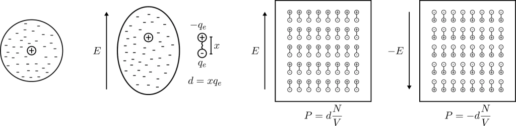
To be more precise, spontaneous emission (from a linearly-polarised dipole-allowed transition) follows the radiation pattern of an oscillating electric dipole, similar to that of a basic antenna. Recall that a radiating dipole is two opposite charges oscillating about each other on a fixed axis.

The fact that dipoles come up again here is not a coincidence. The rules of dipole-allowed transitions and dipole radiation stem from the same approximation that the wavelength of the emitted light is much greater than the physical size of the atom.

On the left, we show the electric field generated by an oscillating dipole oriented in the vertical direction. We see that, apart from the direction of the dipole, the field propagates rather isotropically, and there is no preferred direction in the horizontal plane. This is essentially because the system has rotational symmetry.

If we look far away from the dipole, we can calculate the optical intensity that is emitted in space for every direction. This graph gives us the probability per steradian that a single photon is emitted at every angle. The redder the colour, the more likely a photon will emerge in that direction.

It should be rather obvious why the above figure is bad for us. To collect all the photons into a light-guiding structure like an optical fibre, we would require an impossible system of lenses and mirrors to redirect all the emission back into the fibre.

And if we lose a large portion of the emitted photons, our deterministic source becomes a low-brightness one, limiting the scalability of our quantum protocols.

The Purcell effect

To help us collect more photons from atoms, we can rely on an amazing fact of optics: the lifetime and radiation pattern of an emitter depend on its surrounding dielectric environment, a phenomenon called the Purcell effect. In fact, the radiation pattern we have shown above is only true for an atom placed in a homogeneous medium.

You might think: “Well, that sounds trivial. If I put an optical element like a lens in front of the atom, I am guaranteed to change it’s emission pattern in some way”. And indeed you would be right, but here we are looking at something a little more subtle.

We mentioned above that spontaneous emission is caused by vacuum field fluctuations. It turns out we can engineer the strength of these fluctuations at the position of the atom to accelerate or slow down spontaneous emission in certain directions. To do this, we have to build structures around the atom which are on the scale of the emitted light’s wavelength (λ).

Let’s look at an example: the emitter placed in between two blocks of high refractive-index material (like gallium arsenide — GaAs).

The important parameter here is the Purcell factor: the ratio of the emitter’s lifetime in the structure divided by its lifetime in the bulk material (here it’s just air). As the distance between the blocks (d) decreases, the lifetime of the emitter varies widely (as quantified by the Purcell factor). What’s going on?

Optical modes

The magnitude of the vacuum field fluctuations depends on a couple of things. First, it depends on the number of solutions there are to Maxwell’s equations at the frequency of the emitter (the so-called density of optical modes). With an increasing number of available modes, there are more paths by which light can get emitted by the atom, and spontaneous emission is sped up.

Secondly, we have to consider how localised the electric field fluctuations of the modes are. An optical mode that is spread out in space does not induce strong vacuum fluctuations at one particular position. Whereas a localised mode concentrates its vacuum field where it is confined in space.

If one particular mode has larger local fluctuations than others, the atom preferentially decays by emitting light into this mode (larger fluctuations translate to high decay rates). The radiation profile is therefore changed because the emission will mostly resemble the profile of the dominant mode.

This is what we are seeing in the above experiment. As the separation between the two blocks decreases, cavity modes come in and out of resonance with the emitter. Cavities are dielectric structures which trap light using an arrangement of mirrors. Here, the cavity is formed from the reflections off the high-index material causing the light to bounce back and forth in the air.

Cavity modes only appears at the frequency of the emitter when we can approximately fit an integer number of half-wavelengths between the blocks, creating a standing-wave pattern in their electric field profile.

In our example however, we only see those modes with an integer number of full-wavelengths. This is because the other modes do not induce any electric field fluctuations exactly at the middle point between the blocks, where we placed our emitter. There is a node in their standing wave pattern. Therefore, no spontaneous emission from the atom goes into these modes, and they don’t affect its lifetime.

In contrast, modes with an integer number of full-wavelengths between the mirrors have the maximum of their fluctuations at the centre (anti-node of the standing wave). Therefore, they strongly affect the lifetime of the emitter and its radiation pattern.

Trapping light

By trapping light with mirrors, we have seen how a cavity mode can induce strong vacuum fluctuations at the position of an atom, and therefore funnel its spontaneous emission in a desired direction. It is important to note that the confinement of cavity modes not only depends on how close the mirrors are to each other, but also on how long the light stays inside the cavity. A “leaky” cavity that does not trap light for a long time also does not induce strong vacuum fluctuations.

The cavity we have studied above can only trap light in the vertical direction. We see that the modes have an infinite extent in the horizontal plane because of the continuous translational symmetry. In addition, they do a rather poor job at that. The reflectivity between air and GaAs is only about 30%, meaning that on each bounce 70% of the light is lost upwards or downwards.

So first, we could use better mirrors. A great way to build a mirror is to alternate thin layers of high and low refractive-index materials. These so-called Bragg mirrors can be engineered to have extremely high reflectivity at chosen wavelengths. This is achieved by making sure that each layer fits a quarter-wavelength of light, so that reflections of all the interfaces interfere constructively.

Next, we have to confine the mode in 3D. One way to do that is to curve one (or the two) Bragg mirrors to compensate for the diffraction of light inside the cavity. Our preferred method is to structure the stack of layers into micropillars. The high refractive-index contrast between the pillar and the surrounding air confines the light inside the pillar due to index-guiding (this is similar to the mechanism by which light is guided by an optical fibre).

By making these structures, we get cavity modes that are highly localised and that trap light for a long time. If an atom is placed at an anti-node of the cavity’s electric field, the probability of the emission going into the cavity mode will be much greater than that of the atom emitting in a random direction.

The final piece of the puzzle is what happens to the single-photon once it has been emitted by the atom and is trapped inside the cavity. The Bragg mirrors are designed to keep the light in for a long time, so the photons will mostly leave the cavity from the sides in random directions. This defeats the point of having a cavity in the first place!

To design a good single-photon source, we have to make one mirror less reflective than the other (with less Bragg layers for example) so that the photons preferentially leave the cavity through that mirror only. This is how we achieve near-perfect directionality of the source. Finally, by placing a fibre close to the output mirror, we can then collect the emitted single-photons with high probability.

Note however, that this is a compromise. By reducing the reflectivity of one mirror, the mode of the cavity is not as long-lived, which reduces the vacuum-field fluctuations and therefore decreases the probability that the atom emits into the cavity mode in the first place. Careful engineering of the structure has to be made to strike the right balance.

Quantum dots

It is a hard technological challenge to build the microstructures for the efficient collection of photons. An even harder task is to place an atom at the exact spot where the vacuum-field fluctuations of the cavity mode are at their maximum. While this can be done with single atoms in a vacuum, this involves a very complex procedure and bulky ancillary equipment.

Trapping electrons

Another way to proceed is to find quantum emitters directly in the solid-state. In the last few decades, a number of ways have been found to isolate the quantum energy levels of single electrons inside materials. The approach that we are leveraging is that of quantum dots.

Quantum dots are small islands of low-bandgap semiconductor material, surrounded by a higher bandgap semiconductor. Because of the difference in bandgap, some electronic states can only exist inside the low-bandgap material. The confinement of electronic states to a few nanometres creates discrete quantum states in a way that is very similar to the classic particle in a box model in quantum mechanics.

This arrangement gives us access to bound electronic states very much like an atom does. That is why quantum dots are sometimes referred to as artificial atoms in the solid-state.

Quantum dots are small islands of low-bandgap semiconductor material, surrounded by a higher bandgap semiconductor. Because of the difference in bandgap, some electronic states can only exist inside the low-bandgap material. The confinement of electronic states to a few nanometres creates discrete quantum states in a way that is very similar to the classic particle in a box model in quantum mechanics.

This arrangement gives us access to bound electronic states very much like an atom does. That is why quantum dots are sometimes referred to as artificial atoms in the solid-state.

We can then use the same procedure described above to generate single-photons from these states. In this case, we use a pulse laser to promote one electron from the highest occupied state in the conduction band of the dot to the lowest unoccupied state in its valence band.

Compared to the hydrogen atom, the absence of an electron in the valence band is more significant. This ‘hole’ acts as its own quasiparticle, and the effect of the laser pulse is to create a bound state of an electron and a hole, called an exciton (another quasiparticle). The exciton doesn’t live forever. The vacuum field fluctuations cause the electron to recombine with the hole and in doing so a single-photon is created.

Suppressing vibrations

The electronic levels are not completely isolated from the solid-state environment there are in. The most important source of noise comes from temperature: the jiggling of the atoms in the semiconductor.

Temperature affects the quantum dots in a couple of ways. First, the presence of vibrations in the crystal’s lattice adds an uncertainty in the energy difference between the electronic levels (technically, they induce decoherence of the energy levels). This has a detrimental effect on the indistinguishability of the emitted photons which will also have this added uncertainty in their frequencies.

The second effect is that the emitter can emit (or absorb) vibrations of the surrounding crystal during the photon emission process. Because the vibrations carry energy, the emitted photons will again have very different frequencies from one emission event to the other, reducing indistinguishability.

The solution to this is to cool the sample to cryogenic temperatures to get rid of the vibrations inside the material. For quantum dot emitters, cooling the samples between 4K and 8K is sufficient to suppress the thermal noise. This is the realm of closed-cycle cryostats, which are much less demanding than the more complicated dilution refrigerators.

Suppressing the laser

Another important consideration for quantum emitters is how to separate the emitted photons from the laser pulses. If we cannot distinguish between the two, the single-photon output is simply drowned out by the laser noise.

Typically, it’s very hard to completely avoid laser light reaching the output of the single-photon source. A good solution here is to use an additional energy level of our quantum emitter.

The key is to find two optical transitions which are separated in frequency (or addressed by orthogonal polarisations of light) such that we can filter out the laser (using optical filters or polarisers) from the single-photons at the output. The excited states must be connected in some way to efficiently transfer the electron to the extra state during the laser excitation.

With dots we have access to two different ways to do that. First, we can use the solid-state environment to our advantage by leveraging the coupling of the emitters to the vibrations of the crystal. By using non-resonant laser pulses, we can force the emission of an acoustic phonon to efficiently prepare an exciton.

The second option we have with quantum dots is to use two electronic states which interact with orthogonal polarizations of light. This is a particularly good method when combined with elliptical cavities.

Putting everything together

At Quandela we benefit from decades of fundamental research in quantum dot semiconductor technology. This allows us to bring all the elements together to fabricate bright sources of indistinguishable single-photons.

Importantly, we use a unique method (developed in the lab of our founders) to deterministically place single quantum-dots at the maximum of the vacuum-field fluctuations of micropillar cavities. In this way, we make the most out of the Purcell effect.

In the figure above, we show a 3D rendering of our single-photon sources. As discussed above, they consist of a quantum dot at the anti-node of a long-lived cavity mode which preferentially leaks through the top mirror towards an output fibre.

The ‘cross’ frame around the pillar cavity is there to make electrical connections to the top and bottom of the semiconductor stack. This allows us to control the electric environment of the dots and tune its emission wavelength with the Stark effect.

With the current generation of devices, we simultaneously achieve an in-fibre brightness of > 30%, a g⑵ < 0.05 and a HOM visibility > 90% (see part 1). With these state-of-the-art performances, we believe that large-scale quantum photonics applications are within reach.

A quick note on scalability

More complex applications in quantum photonics require multiple photons to arrive simultaneously on a chip. The obvious route here is to have multiple sources firing at the same time to provide single-photons in multiple input fibres.

While it is generally more difficult for remote sources to generate identical photons (i.e. with perfect HOM visibility), recent results suggest that the reproducibility of our fabrication process is the key to large-scale fabrication of identical sources.

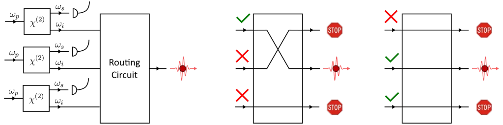
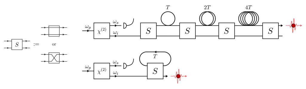
Additionally, we can use active temporal‐to‐spatial demultiplexing to take advantage of the indistinguishability of the photons coming from the same source. This technique can be thought as the inverse of the temporal multiplexing that we saw in part 2 for spontaneous pair-sources.

Starting from a train of single-photons, we switch and delay some of the photons to get several spatial inputs. With a demultiplexer, we reduce the repetition rate of our source to achieve synchronised inputs. The n-photon coincidence rate is then given by

where (as we defined in part 1) μ is the detection efficiency, B the source efficiency and 𝜂 is the demultiplexer efficiency. R is the repetition rate of the laser pulses.

Conclusion

In this series, we have reviewed the state-of-the-art technology for producing single-photons on demand. We have explored in some detail the underlying principles of spontaneous-parametric-down-conversion and atom-like quantum emitters and highlighted their differences.

At Quandela, we feel that quantum-dot sources have great potential for the miniaturisation and scalability of optical-qubit generators. We are working hard to improve their performances and to make them accessible to a wider academic and industrial audience.

If you would like to know more about our technology please email contact@quandela.com or visit our website https://quandela.com/ . If you would like to join our mission to build the world brightest sources of optical qubits, please have a look at our job openings at https://apply.workable.com/quandela/ .

Article by Sebastien Boissier

Heralded Sources and Multiplexing

Welcome to part two of our series on single-photon sources. Here, we will discuss one possible route for single-photon generation: spontaneous photon-pair sources.

Non-linear optics

To understand spontaneous photon-pair sources we have to delve into how dielectric material react to light. Classically, light is nothing but the synchronised oscillations of electric and magnetic fields. And dielectrics are electrical insulators which can be polarised by an electric field. Let’s try to unpack these concepts.

When an electric field E is applied to a dielectric material, the electrons within the material’s atoms are pulled away from their respective nuclei but without being able to escape (because dielectric materials are insulators). This creates many dipoles (pairs of positive and negative charges separated by a small distance) and we say that the material is polarised.

The macroscopic strength of these dipoles is described by the polarisation density P which is given by P = x * qₑ * N/V where x is the separation between to charges, qₑ is the negative charge (assuming the charges are opposite but equal in magnitude) and N/V is the density of dipoles (number of dipoles per unit volume).

Let’s now assume we have a perfectly monochromatic laser beam oscillating with an angular frequency ω and traveling through the dielectric. In complex notation we can write this as

where c.c. is the complex conjugate of the term in front. In response to the oscillating electric field, the electrons and nuclei also start to oscillate, and we get a bunch of oscillating dipoles which in turn lead to a macroscopic polarisation density P(t) that oscillates. It is typically assumed that P(t) depends linearly on the external electric field, so that

where the constant of proportionality ꭓ⑴ is known as the linear susceptibility of the material and 𝜖₀ is the permittivity of free space. The important take-away here is that the dipoles oscillate at the same frequency than the laser.

What’s more, oscillating dipoles are nothing but accelerating charges which themselves emit electromagnetic radiation. It turns out that the dipoles act as a source of light Eₚₒₗ(t) which oscillates at the same frequency as P(t). This new field then gets added to the external driving field.

We therefore have the following string of cause-and-effect Eₗₐₛₑᵣ(t) → P(t) → Eₚₒₗ(t) which produces the output field Eₗₐₛₑᵣ(t)+Eₚₒₗ(t) where the two components oscillate at the same frequency.

In some dielectrics and at high driving power (large Eₗₐₛₑᵣ), the linear relationship between Eₗₐₛₑᵣ(t) and P(t) breaks down. We now enter the nonlinear regime where the relationship is better approximated by adding extra terms in the power series expansion like so

Note that ꭓ⑵ and ꭓ⑶ are typically a LOT smaller than ꭓ⑴ in magnitude. Focusing on the ꭓ⑵ non-linearity and expanding the squared term we get

In this regime, the dipoles not only oscillate at the frequency of the driving laser but also pick up another frequency component at 2ω. The result is that light is emitted at a different frequency than what had been sent in the material. In this case, we get second-harmonic generation.

So what is happening at the level of the photons? Recall that the energy of a photon is given by ħω where ħ is the reduced Planck’s constant. Here we’re assuming that the material is transparent (that it does not absorb energy), so in order to conserve energy two laser photons at frequency ω must be absorbed to generate a photon at frequency 2ω.

Another interesting thing happens when we drive the dielectric material with two laser beams at different frequencies:

Again, focusing on the ꭓ⑵ non-linearity and expanding the squared term, we get terms that oscillate at frequencies ω₁+ω₂ and ω₂-ω₁ (assuming ω₂>ω₁). This is called sum- and difference-frequency generation. Sum-frequency generation is easily understood as one photon from each driving field being absorbed to produce a photon at ω₁+ω₂.

Difference-frequency generation is a little more interesting. During this process, one photon at the pump frequency ω₂ is absorbed and two photons are emitted, one at the driving frequency ω₁ (the signal photon) and the other at ω₂-ω₁ (the idler photon).

Spontaneous parametric down‑conversion

If we attenuated the signal field (ω₁) down to zero, we would not expect any difference-frequency generation to occur. However, the electromagnetic vacuum is not completely empty and at the quantum level there are vacuum fluctuations. These fluctuations correspond to the momentary appearance of particles (in our case photons) out of empty space, as allowed by the uncertainty principle.

It turns out that vacuum fluctuations cause difference-frequency generation in ꭓ⑵ dielectrics without the presence of a signal field. This process is called spontaneous parametric down‑conversion and leads to one photon in the pump field being absorbed and a photon pair being emitted. Parametric just means that no energy is absorbed by the material, and the process is spontaneous because we cannot control when and where in the crystal the down‑conversion will occur (like all the other nonlinear processes).

Because we don’t have a second reference frequency any more, it’s fair to ask at what frequencies the photons will emerge. In addition to respecting conservation of energy, the photons involved in the down‑conversion process must also obey conservation of momentum. The momentum of a photon is given by ħk where |k|= n(ω) * ω / c is called the wavevector and it depends on the material’s refractive index n at the frequency of the photon (c is the speed of light).

Momentum conservation dictates that k(ωₚ)=k(ωₛ)+k(ωᵢ) (where the subscripts p, s and i correspond to the pump, signal and idler photons respectively), and because of material dispersion and birefringence this condition is only satisfied for certain frequencies, directions and polarisation of the photons (and they need not be the same for the signal and idler).

Conservation of momentum is also referred to more broadly as phase-matching. In general, the properties of the signal and idler photons satisfying energy and momentum conservation are usually not the ones we want. To solve this, we must engineer the nonlinear material and the setup to achieve phase-matching for the correct output frequencies. This can be done by birefringent phase-matching, by engineering the dispersion profiles of optical modes and with quasi-phase-matching.

Materials with large ꭓ⑵ coefficients required for spontaneous parametric down‑conversion are usually rather exotic. Common choices are lithium niobate (LiNbO3), potassium titanyl phosphate (KTiOPO4) or aluminum nitride (AlN).

It is also possible to use higher non-linear coefficients to achieve a similar effect. The other popular choice is spontaneous four-wave-mixing in ꭓ⑶ materials. More common materials, like silicon, have large ꭓ⑶ coefficient which makes this process an appealing alternative.

Spontaneous photon-pair sources as emitters of single photons

The discussion so far has been quite removed from the topic of single-photon sources. In this section we finally answer why spontaneous photon-pair sources can be useful in that regard.

Two-mode squeezed-vacuum

First, let’s recall (see part 1 of the series) that sources of single photons have to be triggered. By exciting a ꭓ⑵ dielectric with a continuous laser, spontaneous parametric down‑conversion does not allow us to control the emission time of a photon pair.

A better alternative is to restrict the emission to time slots defined by laser pulses. The nonlinear process can only take place when the laser is “on” and that acts as our trigger. However, we cannot completely control whether a photon-pair is emitted within one laser pulse or if we get multiple pairs.

In fact, if we can separate the down-converted photon from the pump light, the photon-number state that we get in each pulse is (ignoring the spectral, momentum and polarization degrees of freedom)

This state is called the two-mode squeezed-vacuum state and the parameter λ (called the squeezing parameter) is a number between 0 and 1 which quantifies the strength of the interaction. λ depends on the ꭓ⑵ nonlinearity, the interaction length and the laser power. Note that the two-mode squeezed-vacuum state is an entangled state in photon number.

Assuming that λ is small, we can approximate the emitted state as

From this, we can directly calculate the probabilities of getting one or two pairs in the time slot defined by a laser pulse. We have to square the amplitudes to get probabilities, so P(1 pair)≈λ² and P(2 pairs)≈λ⁴.

If we separated the signal and idler photons, could we use either of them as a single-photon state? Well, we are not off to a great start because we have some probability of having more than one photon-pair per laser pulse. In fact, if we completely ignored one of the outputs of the down‑conversion process (say the signal photons), the idler photons would have

Remember that a single-photon source needs a g⑵ as close to 0 as possible to avoid errors in our quantum protocols. A g⑵ equal to 2 is bad. In fact, it’s worse than if we had just used strongly attenuated laser pulses directly, which have g⑵=1.

Heralding

This can be redeemed if we use the photon-number entanglement in the two-mode squeezed-vacuum state. The trick is to monitor one of the outputs (say the signal) and record which output pulses have one or more photons. If we detect signal photons in a particular time slot, we now know that there is at least one photon in the idler path.

So, conditioned on the detection of a signal photon (or photons), the state of the idler collapses to the mixed state

where we have used the density matrix formalism. The vacuum component is projected out.

This time, the g⑵ of the idler photon is

And there we have it. By heralding the presence of idler photons with the signal photons, we get a state that approximates a single-photon state asymptomatically better as λ² tends to zero.

However, recall that the probability of getting a single-pair per pulse is also related to λ² (in fact it is equal to λ²) . This is an important compromise we have to make with spontaneous photon-pair sources: we have to keep the brightness of the source low in order for the single-photon purity to be high. It’s a trade-off between scalability and algorithmic errors. For example, if we wanted P(1) to be 10%, then g⑵=0.2 and that’s quite high for a single-photon source.

Note that this can be improved with the use of photon-number resolving detectors, which not only measure if there are photons but also how many. By heralding only the single-photon events in the signal paths (and rejected the vacuum and multi-photon components), we can decrease the g⑵. Even so, the statistics of the two-mode squeezed-vacuum state as such that the theoretical limit for brightness is 25%.

Spectral purity

Heralding is a great way to turn spontaneous photon pair sources into single-photon sources. However, it also creates additional constraints on the nonlinear process. Let’s focus on the frequencies of the emitted photon pair. In general, the emitted state is given by

where f(ωₛ, ωᵢ) is called the joint-spectral-amplitude. If f(ωₛ, ωᵢ) is not factorable — i.e. f(ωₛ, ωᵢ)≠ f(ωₛ)* f(ωᵢ) — the photons are entangled in frequency and measuring the signal photon collapses the idler to a mixed state, generally written

Mixed states in frequency are not a problem for photon purity. A single-photon, regardless of its frequency state, will only be measured at one output of a beam-splitter, and therefore has g⑵=0 (see part 1). However, it is bad for its Hong–Ou–Mandel visibility. A mixed state essentially means we have classical probabilities pₙ of getting different quantum states every time. And distinguishable states will not produce perfect interference on a beam-splitter (again, see part 1). In general, the detection of the signal photon must teach us nothing about the state of the idler photon except for its presence.

To have a spectrally-pure idler state, we have to work harder to engineer a factorable joint-spectral-amplitude. This can be done with group-velocity matching and apodization of the joint spectral amplitude by engineering the profile of the nonlinear medium. Another good method is to further engineer waveguide modes and using long interaction lengths.

Failing to produce a factorable spectrum, we can always filter the output photons to reject all possible frequency states but one. While this approach improves spectral purity and therefore indistinguishability, it comes at the cost of reducing the brightness of the source and that compromises its scalability even more.

Multiplexing

The balance between brightness and single-photon purity seems to be a major hurdle for spontaneous photon-pair sources. Is this the end of the story? No, because we can improve the efficiency of these sources by multiplexing.

At its core, multiplexing is a simple idea. Instead of using just one time-bin of one photon-pair source, we combine multiple sources (spatial multiplexing) or incorporate several time-bins of the same source (temporal multiplexing) to produce a better single-photon source. We consume more resources for better performance. Let’s quickly talk about both options.

Spatial Multiplexing

With spatial multiplexing, we first have to build a number of identical photon-pair sources. It is important that all the heralded single-photon outputs are the same or the indistinguishability of the multiplexed source will suffer.

Once that’s done, the output of the sources are connected to a reconfigurable routing-circuit (a multiplexer). All the sources are then pumped simultaneously with laser pulses and we monitor the emission of signal photons. We then pick one of the sources which has fired and route its now-heralded idler photon to the output of the circuit.

Because we have multiple sources working together, the probability that at least one fires can be a lot greater that the brightness of the individual sources. In fact, assuming a perfect routing circuit the brightness is improved by

where B₁ is the brightness of the sources and N is the number of sources hooked-up to the routing circuit.

Things now look at lot better, but we do have to consume a lot of resources. Say we want a source with g⑵=0.05 (that’s not bad for the state-of-art), then B₁ ≅ P(1) = 2.5% and we need at least 15 sources for a final brightness of 30% (28 for 50% and 91 for 90%).

Temporal Multiplexing

The other variant of this technique is temporal multiplexing. Here, we use contiguous time-bins of the same source (recall that we pump the sources at regular time intervals). We simply wait for the source to fire in one of the time-bins and delay the heralded idler-photon accordingly so that it leaves the circuit in a known time-bin.

The overall effect is the same as for spatial multiplexing but N is now the number of time-bins that we use. One key advantage of temporal multiplexing is that sequentially emitted photons of the same source are usually more similar than those emitted by different sources, which helps with indistinguishability. The price we pay however is a decrease in the repetition rate of our source which goes from R to R / N.

Repetition rates are important in quantum photonics because experiments are usually probabilistic. We typically known when a particular run has succeeded but we could wait a while for that to happen. The ability to perform the experiment as often as possible is therefore desirable. This is what we are sacrificing with time-multiplexing.

We could also have anything in between full-temporal and full-spatial multiplexing depending on the scarcity of our two resources (experiment time vs number of sources).

Outlook

As can be seen in figures above, multiplexing can be wasteful. As we add more sources (or time-bins) to boost the brightness, we also increase the probability that two or more sources fire in the same multiplexing circuit. Unfortunately, we have to discard these photons because trying to route them to a second exit (or time-bin) will just add complexity and result in an additional source which has a poor brightness.

One interesting idea to improve this is that of relative multiplexing. In this scheme, we do not force the sources to always emit in the same exits or time-bins. Instead, we correct the relative distance (in space or in time) between photons that have been heralded. By using more of the emitted photons, we can reduce hardware complexity while improving coincidence counts.

It must be said however that multiplexing relies on the ability to integrate high-performing photonic components at scale. To implement a routing circuit, we must have access to optical switches, delay lines, single-photon detectors, fast electronics, etc… At present, photonic components can be lossy and/or slow to operate. This limits the performance of multiplexing, and we have to use even more hardware to reach the required improvement in brightness.

Summary

In summary, we have looked at how spontaneous photon-pair sources can generate single photons. We have seen how these sources are probabilistic, in the sense that we cannot completely eliminate the probability of multi-photon emission. In addition, it is only when the presence of one photon is heralded by the detection of the other that these sources become useful for single-photon generation.

We also described how the brightness of these heralded sources has to be kept low in order for the purity of the emission to be high. This can be remedied by multiplexing, but at the cost of multiplying the number of components, and therefore limiting the scalability in the long run.

Heralded photon-pair sources are very much still an active and ongoing topic of research, both theoretically and experimentally. An up-to-date review of the topic can be found here.

Next up

In the next post we will discuss a different approach to creating single-photons using deterministic quantum emitters. Compared to heralded pair-sources, deterministic sources have taken a longer time to mature and they now form the core of Quandela’s technology.