


Article by Lucija Grba
Linear optical quantum computation uses photons as carriers of information (i.e. qubits) in an optical circuit with beam splitters and phase shifters that process this information. You can read more about how optical quantum computing works here.
Let different outputs of an optical quantum circuit correspond to different spending models one can obtain with a specific number of photons corresponding to their limited budget. Naturally, the more spending models we have access to, the more options we have to choose from and therefore have a higher likelihood of making an optimal choice. If before we had the categories ‘food’ and ‘travelling’, we will surely benefit from branching out these categories into ‘groceries’, ‘fast food’, ‘restaurants’ and ‘flights’, ‘public transportation’ etc. While we may have given a high importance to the category ‘food’ before as it is essential to our survival, we can now identify that some categories like ‘fast food’ and ‘restaurants’ aren’t as essential as ‘groceries’ so we have a higher chance of making better choices with a limited budget.
For the creation of a good photon spending model, it’s important not only to know how many photons there are in a budget (entered the circuit) and where they were found in the end (on which output modes). It’s important to also quantify the photon expenses on each mode (how many photons are found in which output mode), so you have a better chance of reaching that photon distribution you’re looking for.
Are you looking for a way to do more complex computations with a limited photon budget but you find yourself not knowing your photon distribution at the end of your computation? Fear not, we have you covered! Keep reading to discover how to make the most of your photons with our new feature — pseudo photon number resolution (PPNR or pseudo PNR).
1. Why is PNR important?
The use of photons as quantum processing units has an advantage of satisfying 5 DiVincenzo conditions for building a quantum computer (remind yourself of these by reading this short article). It also gives access to a truncated Fock space, that is larger than the qubit space. We measure this difference by the size of the Hilbert spaces that describe them mathematically. You can read more about the difference between these in one of our previous articles here.
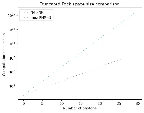
In short, using the photonic Fock space gives us a scaling advantage. With the same number of photons, the Fock space is much larger than the qubit space, and therefore allows us to construct and work within a greater computational space. Essentially, we can do more with less, helping you make the most of your photons! This can be viewed as the expansion of the number of categories we consider for our photon spending model we talked about earlier.
We previously stated that we couldn’t count the number of photons in a single output mode with perfect accuracy, limiting our access to some states in the Fock space, i.e. a truncated Fock space. While perfect accuracy is still difficult to achieve, we are happy to share that we have made a great stride towards it!
Perceval users can now configure their modes, declaring them photon number resolving or not. This is an optional feature already introduced in our software and ready for use!
2. PNR integration
You’ve probably heard about microprocessors or classical processing units (CPUs). Think of them as the brains of a computer, processing and analysing information using classical operations. They are connected to other parts of the computer through pins, some of which have a predefined function (meaning that they can only perform one function, such as RESET pins) while others are configurable. These are called general purpose input/output (GPIO) and are much more useful.
An analogy of the same idea of configurable ports can be applied on optical devices in a quantum processing unit (QPU). A QPU differs from a CPU in the way its computations are performed, harnessing the power of physical behaviours occurring with quantum particles.
Photon detection works based on a grid — changing the position and number of photons found in each mode of the grid changes the state of the system (spending model considered). This is why having access to a PNR detector is imperative to achieving high fidelity. A single photon detector (SPD) would only be able to tell us whether it detected any photons at all (giving us the output 1) or none at all (outputting 0). You can visualise the difference between the capabilities of PNR and SPD below.
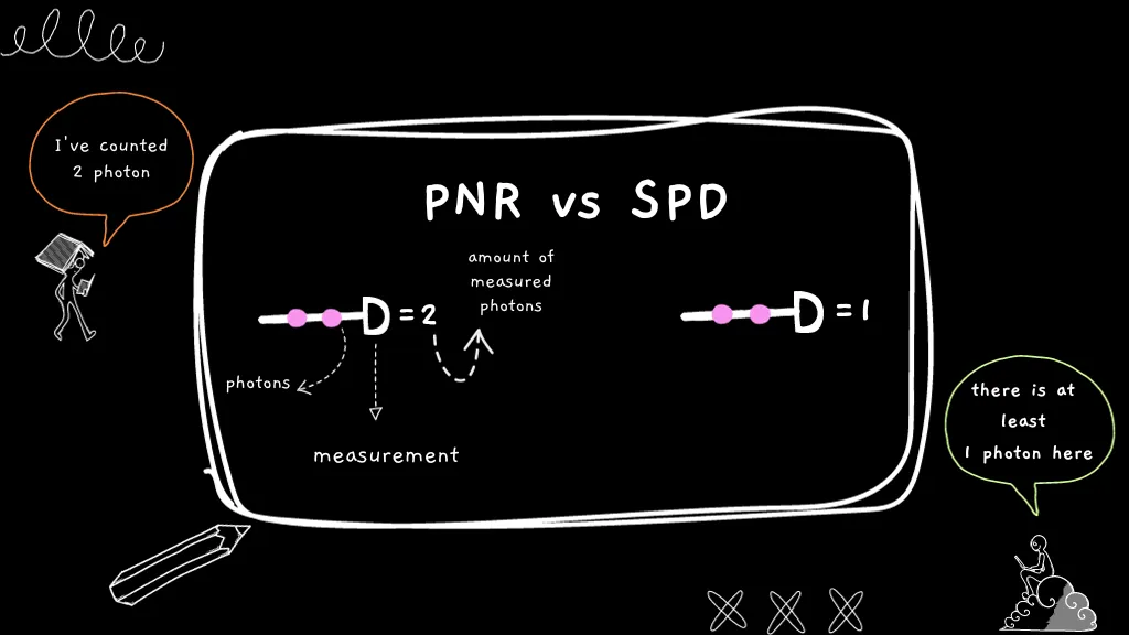
In simple terms, PNR detectors allow you to analyse your photon distribution better (as they have access to more spending models) so you naturally have a better chance of finding that distribution you’ve been dreaming of obtaining. Now you might be wondering: how is PNR achieved in a photonic quantum computer?
Our newest feature uses balanced beam splitters attached to the modes the user has declared PNR. Recall that a beam splitter is an optical device containing 2 input modes and 2 output modes. It controls the direction of the photons that pass through it. A balanced beam splitter gives a photon entered through either of the inputs a 50% chance of ending up in either of the outputs (the choice is random), as it can either reflect off the beam splitter or be transmitted through it.
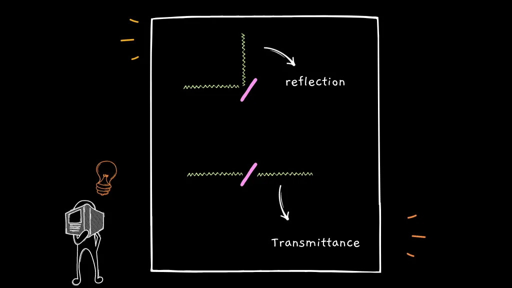
Imagine a mode containing 2 photons connected to our PPNR detector. Reaching a balanced beam splitter, these photons will end up either taking the same route and will therefore be found in the same mode with a 50% probability, or they will each go their way and be found in separate modes with a 50% probability.
There are 4 different ways 2 photons might travel through a beam splitter, each equally likely to occur (each with 25% probability)
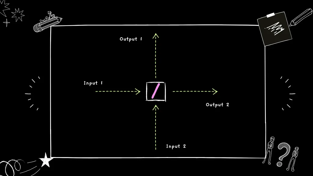
Case 1: Input 1 and input 2 were both reflected and came out the outputs 1 and 2 respectively.
Case 2: Input 1 was reflected and input 2 was transmitted so they both ended up in output 1.
Case 3: Input 1 was transmitted and input 2 was reflected so they both ended up in output 2.
Case 4: Input 1 and input 2 were both transmitted and came out the outputs 2 and 1 respectively.
Since photons are indistinguishable, we recognise that there’s a 50% probability of the photons splitting up and 50% probability of them ending up in the same mode.
We call this pseudo PNR because we obtain the photon distribution probabilistically and not deterministically. In simple terms, we do not have full control over whether a photon gets reflected or transmitted as this happens randomly, with a certain probability (50%).
We constructed a set-up that manipulates how our photons travel and gives us a good chance of counting 2 photons if they are travelling together in a single mode. An example of a non-pseudo PNR would be PNR that deterministically determines the number of photons in a mode by measuring the intensity of light. The more photons are found in a mode, the stronger their light will be. If we can deterministically measure the brightness, we are 100% confident in the photon count and this would be true PNR.
For now, PPNR can only be used on the first 3 modes of our QPU and its simulator, but this can also help us infer knowledge about other modes. You can test its performance for an up to 2-photon number resolution with 50% accuracy. The feature can easily be implemented in a single line of code, as shown in the picture below.

Stay tuned for future releases on more modes!
This is a great step forward, broadening the limits of what is possible to do in our framework and paving the way for some very exciting applications. In quantum machine learning, it allows us to work with more complex learning models as we are able to work in a larger computational space (Fock space). You can find a simple visual explanation for why that is the case here. Furthermore, in quantum algorithms for classification (VQC), access to PNR allows the creation of a highly expressive ansatz, automatically increasing the complexity of the circuit without increasing the number of photons used. You can explore how and why we use VQC on our very own QPU Ascella here.
So, what are you waiting for? Uncover the full potential of our new feature and make the most of your photons!
If you are interested to find out more about our technology, our solutions or job opportunities visit quandela.com