What are Surface codes?
The data that is used by a quantum computer to perform algorithms can be affected by noise. It is thus expected that quantum error correction will be necessary to run long quantum algorithms. There are many ways to encode data into a quantum system, but, currently, the most widely used quantum error-correcting code is the Surface Code.
An example of stabiliser code
The surface code is an example of Stabiliser Code. The data is therefore encoded into a multi-qubit system and a set of so-called stabiliser operators leave the system unchanged when applied. Measuring these operators can be used to detect errors and recover the data.
In the case of the surface code, qubits are associated with edges of a square lattice. There are two types of stabiliser operators respectively associated to the “plaquettes” of the lattice and its “stars”. Examples of such plaquette and star operators are shown on the figure below. This enables to encode 1 logical qubit into a grid of L-by-L physical qubits.
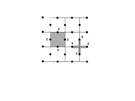
Figure: Examples of plaquette and star stabiliser of the planar surface code. For every plaquette of the square lattice, applying a Pauli-Z on all the qubits involved in the plaquette leaves the encoded information unchanged. Likewise, for every star in the square lattice, applying a Pauli -X on all the qubits involved in the star leaves the encoded information unchanged.
Advantages of the surface code
The surface code has been studied for many years and as a result probably is the most well-understood quantum error-correcting code. Methods to implement the surface code are well-known and small instances of surface codes have already been implemented experimentally.
Stabiliser codes are very useful because there exist known techniques to initialize them and detect errors with them. This is done by measuring the stabilisers. The lower the number of qubits involved in each stabiliser is, the easier it is to implement the measurement in practice. In the surface code, every stabiliser measurement involves at most 4 qubits, no matter the size of the surface code (=its number of physical qubits). This is an important asset of that code. Moreover, it is easier to perform stabiliser measurements when the qubits involved are physically close to one another. In many quantum architecture platforms, this “locality” constrain is very high, and this is the main reason the planar surface code is so popular. Indeed, if the physical qubits are put on a grid, in a planar layout, stabiliser measurements in the surface code only involve qubits that are physically close, as shown on the picture above. The surface code is therefore compatible with architectures offering only local connectivity (meaning that the physical qubits only need to interact with their neighbours). Quandela’s architecture on the other hand allows for high range connectivity so there is no locality constrain, which gives the option to consider other codes, potentially less resource intensive (see “Drawback” section below).
Moreover, methods to implement a universal set of logical gates and hence perform algorithms while correcting the errors with a surface code are also known. Likewise, decoders (used to know which errors occurred) for the surface code are efficient. Finally, the threshold of the surface code family makes is competitive over many other options.
Drawbacks of using a surface code
Despite its important assets, the planar surface code is resource intensive. A grid of L by L physical qubits is required to encode just one logical qubit. When the size of the code grows (which is needed to correct more errors), the encoding rate (= the ratio of the number of logical qubits over that of physical qubits) converges to 0. Likewise, the ratio of the distance of the code (quantifying how many errors the code can correct) over the number of physical qubits also converges to 0. This last point actually is a fundamental limit: the distance rate necessarily vanishes asymptotically for any 2D local code family. An important asset of Quandela’s envisioned fault-tolerant architecture is that it is compatible with codes that are not 2D local, and hence do not suffer from this limitation.
Frequently Asked Questions
- Can it ever happen that you do not detect an error even if one has happened? Yes, it can! If an error affects too many physical qubits, then that error is undetectable. In the surface code, the number of errors that can be corrected is proportional to the size of the code: in a surface code of L by L qubits, then at most (L-1)/2 Pauli errors (=elementary errors) can be corrected.
- What’s the difference between surface code, toric code, planar surface code and rotated surface code? Researchers at Quandela have shown that pair-wise measurements, the main operation needed to implement Floquet codes, are easy to realize on its envisioned hybrid spin-optic architecture, SPOQC. This makes Floquet codes well suited to the platform. Moreover, some numerical simulations indicate that the honeycomb Floquet code, which can be thought of as a “floquetification” of the surface code, performs better on the architecture than the surface code, in terms of threshold.
- How would one perform a computation on a quantum computer where the quantum information is encoded into a Floquet code? In principle, “surface code” is a generic word for any stabilizer code whose X-type and Z-type Pauli stabilizer generators are associated to the stars and plaquettes, respectively, of a cellulation of a two-dimensional surface. Typically, the cellulation considered is a square lattice but one may also consider different lattices such as triangular or hexagonal lattices. In practice, a bit confusingly, the term “surface code” is often used ever as a short-hand for planar surface code or as a synonym of toric code. By definition, a planar surface code is a surface code implemented on a (finite) section of a plane. On the other hand, a toric code is a surface code for which the surface considered is that of a torus. In the bulk, i.e. the interior region of the surface, the stabilizers of a planar surface code on a square lattice are those shown on the figure above, but on the boundaries, one considers weight-3 half-star and half-plaquettes stabilisers. The rotated surface code is very similar to the planar surface code. It shares all the nice features of the planar surface code (in particular its planar layout with local connectivity) with the additional advantage that it uses slightly less qubits than the surface code to correct the same number of errors. In practice, it is therefore often the rotated surface code rather than the planar surface code that is implemented. Its name comes from the fact that its layout in the bulk can be obtained by rotating a planar square-lattice surface code by 45 degrees. The stabilizers only differ on the boundaries.
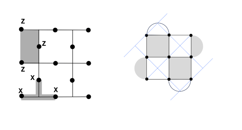
Left: Examples of Z-type half-plaquette stabilizers of the surface code and X-type half-star stabilizers on the boundaries, in a distance-3 planar surface code. Qubits are on the edges of the lattice.
Right: Layout of a distance-3 rotated surface code. Qubits are associated with the vertices of the full-line square lattice. Dark plaquettes are associated with X-type stabilizers and light plaquettes are associated with Z-type stabilizers. On the boundaries, one can see that the stabilizers involve only 2 qubits. The blue dotted-line lattice has been put to show that, in the bulk, the stabilizers can equivalently be seen as Z-type plaquette and X-type star stabilizers, where qubits are now on the edges of the blue lattice. This code uses 9 data qubits, as compared to 13 data qubits for the planar surface code achieving the same distance.