


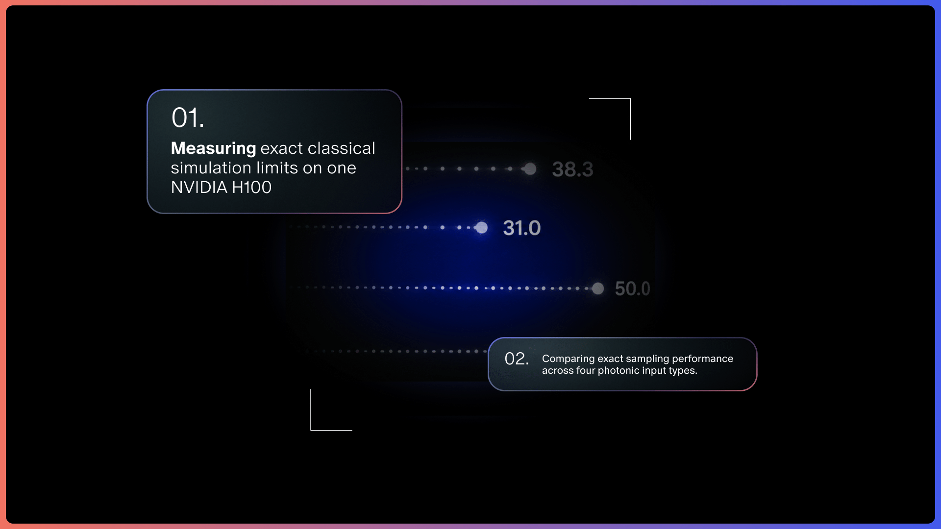
We measured, on one NVIDIA H100 GPU, the device size at which an exact classical sampler still produces one sample per second, for single photons, squeezed light, quantum-emitter trains and several other inputs.
One yardstick for every kind of input: seconds per exact sample, on one fixed machine, on specified instances. Universal interferometers with m = 2n modes; the numbers below are photonic inputs n at one exact sample per second on one NVIDIA H100.
Fifty, sixty, ninety-eight
How many photons does a boson sampler need before a classical computer can no longer follow it? The literature gives answers from 50 to 98 photons. These answers do not contradict each other, because they measure different things. Clifford and Clifford proposed about 50 photons from the cost of their exact sampler. Neville et al. arrived at more than 60 or 70 photons under their own assumptions about source rate, transmission and mode scaling. A fine-grained complexity analysis gave 98 photons and 500 optical elements under specified conjectures. For squeezed light and for loop architectures, the figures quoted are clicks, memory or core-hours, which cannot be converted into a common photon threshold.
None of these numbers tells an engineer what a classical machine can do at the rate a device runs. In our paper we use one yardstick for every kind of input: seconds per exact sample, on one fixed machine, on specified instances.
The simulability frontier
The simulability frontier is the set of device parameters at which the fastest exact sampling algorithm we implemented and evaluated produces a target rate R of samples per second on a fixed machine. Here R is one sample per second and the machine is a NVIDIA H100 GPU.
The axis is the number of photonic inputs n: the input modes of the interferometer that receive light, whether a single photon, one photon of an emitter’s train, a superposition of vacuum and one photon, or a squeezed state. Exact sampling cost grows roughly as βn. As a result, a constant-factor speed-up X moves the frontier by only ln X / ln β photonic inputs. For single photons, a 2× faster kernel adds 1.2 photonic inputs and eight GPUs add 3.5 (we checked this by direct timing). A 16,384-accelerator exascale partition would add 16.2. Reaching 100 photonic inputs with hardware alone would take about 1016 GPUs. A better algorithm acts differently because it changes β itself. On one H100 with the same code substrate, replacing the 2018 Clifford–Clifford algorithm with the 2020 version moves the single-photon frontier from 32.5 to 35.7 photonic inputs. Moving from that implementation to our production NVIDIA CUDA kernel then takes it to 38.3.
Where one H100 stands
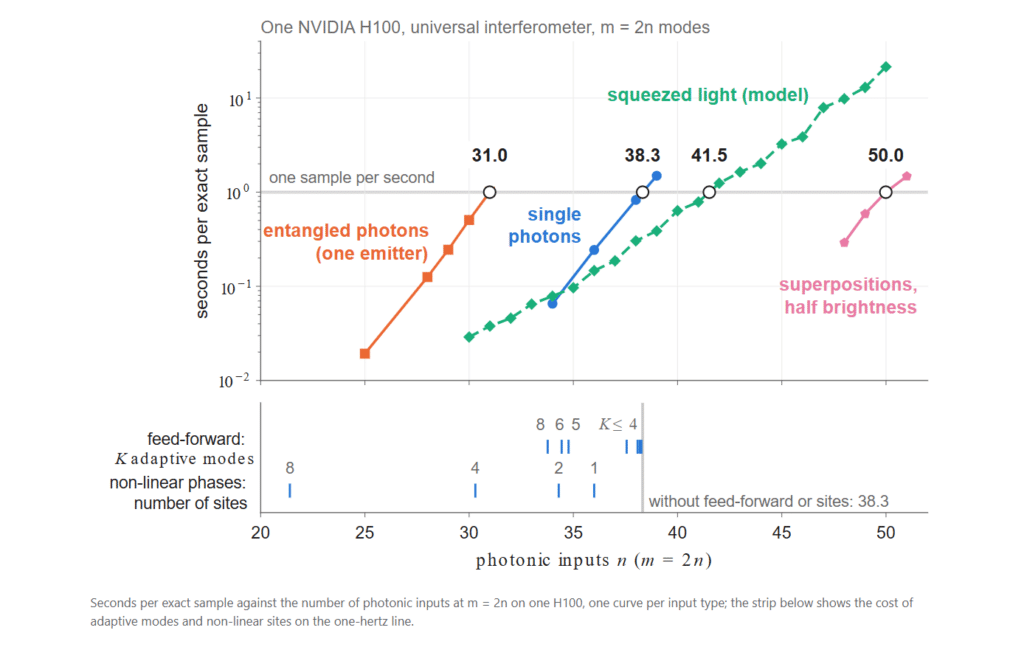
For universal interferometers with m = 2n modes, one exact sample per second on one H100 is reached at:
| Input | Photonic inputs n at 1 sample/s | Basis of estimate |
| Photons from quantum emitters | 31.0 | Measured |
| Single photons | 38.3 | Measured |
| Squeezed inputs, mean photon number 0.5 | 41.5 | Modelled |
| Superposition of vacuum and one photon, half brightness | 50.0 | Measured |
The squeezed-light value is modelled, not measured: it comes from a calibrated timing model of a cost statistic truncated at the photon number that a run of 104 samples reaches.
Measuring every input on the same scale also shows how much each feature of a device costs:
- At fixed brightness, coherence between photon-number branches moves the frontier of the sampler we evaluated by 14.2 photonic inputs.
- For lossless single photons, one non-linear site of phase π/2 moves it by 2.2 photonic inputs.
- Feed-forward on up to three adaptive modes moves it by at most 0.2 photonic inputs.
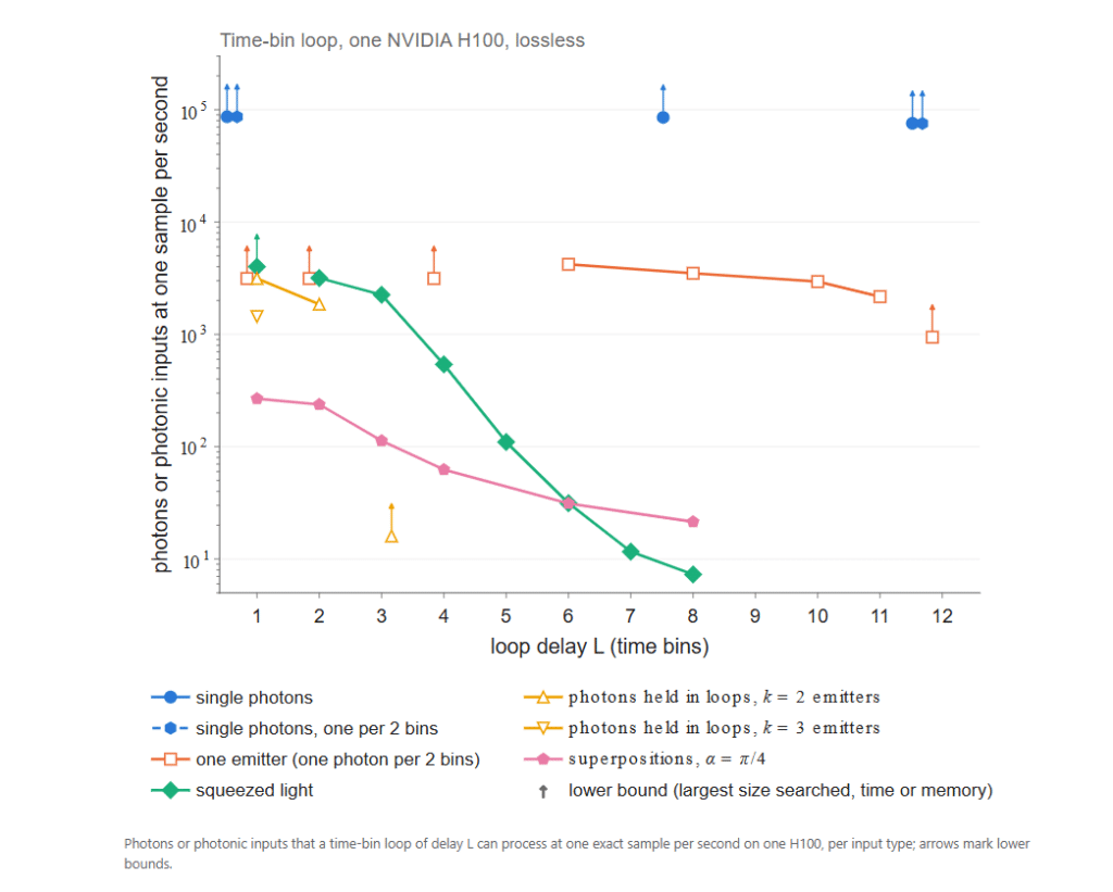
Some devices reuse one interferometer tick by tick on a photon train instead of spreading the train across space. For these, the exponent is no longer the number of photonic inputs but the register carried from tick to tick. For an emitter train, that register is the emitters’ spin register: about 21–22 emitters per tick at one tick per second, extrapolated from 18, whatever the train length. The whole train costs its length times that. For time-bin loops, the frontier becomes a loop delay rather than a photon number.
Three other limits: memory, precision, energy
Rate is not the only resource that limits exact simulation.
Memory limits strong simulation, which writes down every output probability. The largest device whose full output distribution fits as complex64 amplitudes in the 80 GiB of one H100 has 13 single photons at m = 2n. Each doubling of memory adds only 0.36 photon. From 14 photons up to the rate frontier, only a sampler can follow the device.
Arithmetic precision limits any finite-precision implementation of an exact algorithm. Double precision (fp64) keeps the per-step error on the probability weights below 10−3 up to about 55 detected photons for single photons and about 62 for squeezed inputs. Both figures are extrapolated from the true error measured up to 38 photons. Beyond that, the sampler needs double-double arithmetic, which current GPUs do not provide natively. Near that range, the number format sets the frontier rather than the number of GPUs.
Energy puts the classical cost in the units of a quantum energetic advantage, which Soret et al. argue can come before the computational one. At 38 single photons, one exact sample costs about 7.3·10−2 Wh of measured H100 board energy. In their estimate, a photonic device needs about 10−8 Wh.
The library
All of these measurements come from one code base, photonic-engines. It is a GPU library with samplers for single-photon, emitter-generated, photon-number-superposed and squeezed inputs, and for adaptive circuits, single-mode non-linear phases, emitter trains and time-bin loops. Several samplers implement chain rules derived in our methods paper. The library also includes the probability estimator for entangled emitter states from a second companion paper.
Each engine is checked against an independent oracle that shares no code with it. Every engine is timed under the same protocol, and an audit records, row by row, the algorithm, the code path, the statistic and the run behind each number. The strong simulators are differentiable PyTorch code, so output probabilities have gradients with respect to the interferometer and the emitter operators. To our knowledge, it is the fastest public exact sampling code for the modalities it covers on generic, full-depth interferometers. Structured, low-depth circuits have specialised algorithms that this claim does not cover. The library is released under the MIT licence.
What it means for a hardware roadmap
The frontier separates what a faster classical machine can do from what a better algorithm can do. Eight GPUs add 3.5 photonic inputs, and an exascale partition adds 16.2, while an algorithm that lowers β changes the slope itself. On the device side, the same scale shows where effort pays off. It shows which input type is hardest to follow per photonic input, how few photonic inputs adaptivity costs, and why squeezed light and quantum emitters must be compared on the same footing as single photons.
The frontier also shows where a near-term device can outperform one GPU. A three-source entangled device emitting at 1 GHz, with 48 photons in 96 modes and 20 % end-to-end transmission, would need about thirty H100 to reproduce its exact output stream in real time. Each of its samples, taken alone, is still easy: the typical sample has about ten detected photons, far inside the one-hertz frontier.
The frontier is a measured rate. It is neither a wall nor a proof of hardness. It can be re-measured whenever an algorithm, a code or a machine improves, and any exact sampler can be timed against it under the same protocol.
References
- Every number on this page is printed in the frontier paper, arXiv:[frontier ID]; the figures are adapted from its Fig. 1 and its time-bin-loop figure.
- Methods paper (chain rules): J. Senellart, S. Wein and P.-E. Emeriau, arXiv:2611.11044.
- Estimator paper (quantum emitters): J. Senellart and P.-E. Emeriau, arXiv:2611.10500.
- Code: github.com/Quandela/photonic-engines (MIT),
pip install photonic-engines.