Exploring Graph Problems with Single Photons and Linear Optics

Introduction (non-technical summary)

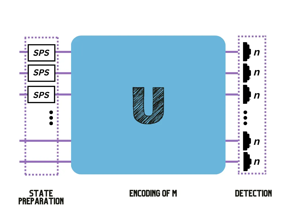
The huge promise offered by quantum computers has led to a surge in theoretical and experimental research in quantum computing, with the goal of developing and optimising quantum hardware and software. Already, many small-scale quantum devices (known commonly as quantum processing units or QPUs) are now publicly available via cloud access worldwide. A few weeks ago, we were delighted to announce Quandela’s first QPU with cloud access — Ascella — a milestone achievement and the first of its kind in Europe.

We are working on developing both quantum hardware and software tailored to our technology. Our QPUs, including Ascella, consist of our extremely high-quality single-photon sources, coupled to linear optical components (or chips), and single photon detectors. We can in principle implement many algorithms on these QPUs, including variational algorithms, quantum machine learning and the usual qubit protocols. Check our Medium profile for more.

This post highlights our latest research: a new important use for our QPUs, namely solving graph problems. Graphs are extremely useful mathematical objects, with applications in fields such as Chemistry, Biochemistry, Computer Science, Finance and Engineering, among many others. Our research shows how to efficiently encode graphs (and more!) into linear optical circuits, in practice by choosing the appropriate QPU parameters, and how to then use the output statistics of our QPUs to solve various graph problems, which we detail below in the technical section. Furthermore, we also show how to accelerate solving these problems using some pre-processing, thereby bringing closer the prospect of achieving a practical quantum advantage for solving graph problems by using our QPUs.

Methods and results

We now take a deeper/more technical look into the workings of our technique. The probability of observing any particular outcome in a linear optical interferometer (say =|n⟩=|n₁,…,nₘ⟩) will depend on the configuration of the interferometer (which can be described by a unitary matrix U) and the input state ( |nᵢₙ⟩=|n₁,ᵢₙ , … , nₘ,ᵢₙ⟩ where nᵢₙ is the number of photons in the iᵗʰ mode in the following way¹ :

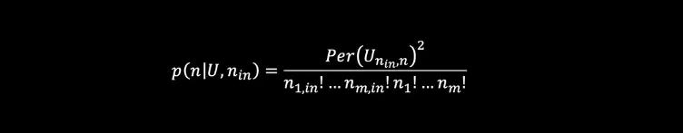
(Unᵢₙ,n is a unitary matrix obtained by modifying U based on the input and output configurations and nᵢₙ.) Hence, the applications for such a device relate closely to a matrix characteristic known as the permanent (Per) — a mathematical function that is classically hard to compute. One of the key techniques we use to make matrix problems solvable using our quantum devices is mapping the solution of a given matrix problem onto a problem involving permanents.

1. Encoding, computing permanental polynomials and number of perfect matchings

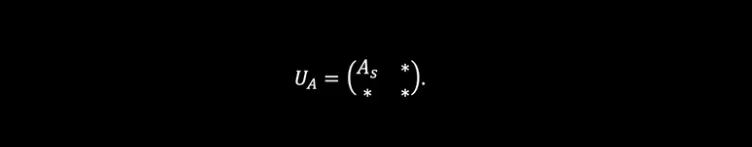
We begin by encoding matrices into our device. Graphs (and many other important structures) can be represented by a matrix. To encode a bounded matrix A, if we consider the singular value decomposition obtaining A = UDV* where D is a diagonal matrix of singular values and take s the largest singular value of A (maximum value of D), we can scale down this matrix into Aₛ = A/s so that we obtain a matrix that has a spectral norm ||Aₛ||≤1. From here, we can make use of the unitary dilation theorem² which shows that we can encode Aₛ onto a matrix which is unitary and has the following block form

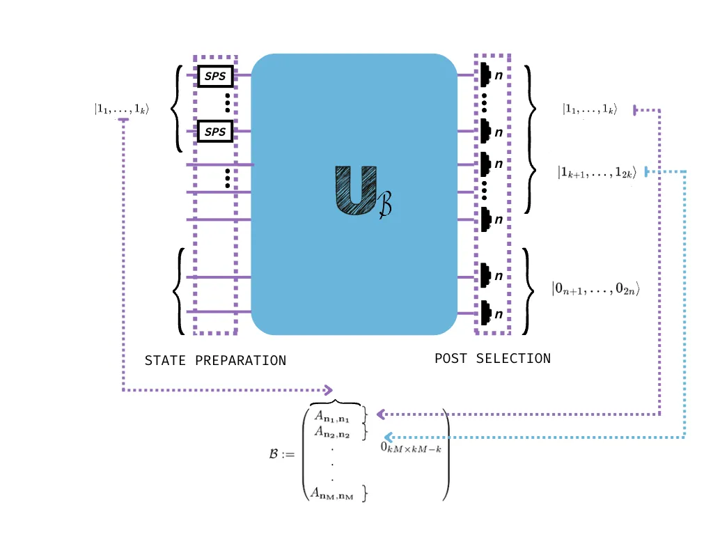
With the appropriate input and output state post-selection, we can estimate the permanent of A by using a setup similar to that of the figure below (see our paper for details³). You can test this estimation for yourself using Perceval, an open software tool developed by Quandela to simulate and run code on a photonic QPU⁴.

2. The k-densest subgraph problem

The densest subgraph problem is the following: given a graph of n nodes, find the subgraph of k nodes which has the highest density. Considering an adjacency matrix A and the cardinality of nodes |V| and edges |E|, we proved in ³ that (when |V| and |E| are even) the permanent is upper bounded by a function Per(A)≤f(|V|,|E|) where f(|V|,|E|) is a monotonically increasing function with the number of edges.

The connection to the densest subgraph problem is natural since the density of a graph defined by the nodes v is:

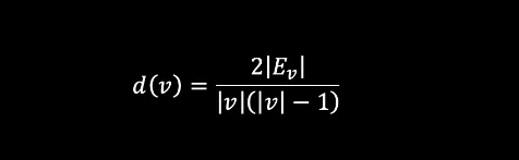
where Eᵥ is the number of edges in that subgraph connecting the nodes v meaning that the density is proportional to the number of edges.

Let n be the number of vertices of a graph G. We are interested in identifying the densest subgraph of G of size k≤n. The main steps of our algorithm³ to compute this are the following:

• Use a classical algorithm⁷ which finds a subset L of size <k of the densest subgraph of G. Then use L as a seed for our algorithm, by constructing a matrix B of all possible subgraphs of size k containing L. In general, this number of possible subgraphs is exponential however, given the classical seed, this number can be reduced to polynomial in some cases³.
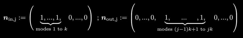
• After constructing the matrix with these possibilities, we choose the appropriate input state and the following post-selection rules:

For clarification, check the figure below.

Each post-selected output computes the permanent of a subgraph, and by the connection established above it follows that the densest one will be outputted the most often, since it has highest permanent value.

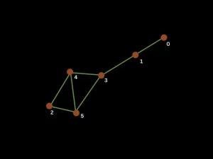
We tested our theory and obtained some results (you can find and reproduce them on this link). Here we present an example. Given a graph G represented in the next figure with node labels, we searched for denser subgraphs of size 3 with minimum number of samples from the linear optical device set to 200.

We tested for different seeds that the classical algorithm might have provided.

1. For this algorithm², 23420000 samples were generated; 200 remained from post selection, all attributed to node group [2,4,5].
2. For this one¹⁰, 21120000 samples were generated; 200 remained from post selection which were distributed over node groups [4,3,5] and [4,2,5] with 115 and 85 samples respectively.

Our algorithm outputted the expected subgraphs from the figure and when it had two equally suited options it correctly outputted both.

3. Graph isomorphism

In our paper³, we prove that computing the permanent of all possible submatrices of the adjacency matrices of two graphs G₁ and G₂ is necessary and sufficient to show that they are isomorphic; however, this is not practical as the number of these computations skyrockets with the number of vertices. One alternative is to import powerful permanent-related tools from the field of graph theory to distinguish non-isomorphic graphs. A powerful distinguisher of non-isomorphic graphs is the Laplacian¹⁰. Starting with an estimation using the permanental polynomials P(x):

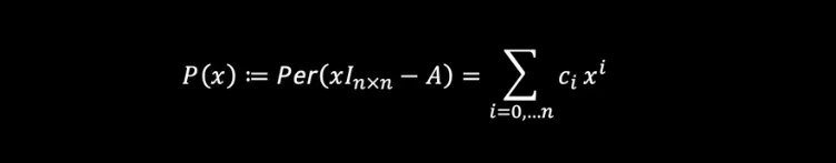
the Laplacian of a graph is given by L(G):= D(G) — A(G) where A(G) is the graph’s adjacency matrix and D(G) is a diagonal matrix where each entry stands for the degree of the corresponding node. Here, in this Laplacian method L(G) replaces A in P(x).

Given two graphs G₁ and G₂, the steps for graph isomorphism are the following:

1. Encode xIₙₓₙ — L(G) for both G₁ and G₂ into unitaries U₁ and U₂ of 2n modes.
2. Compute an estimate of Per (xIₙₓₙ — L(G)) for each graph by using the configuration before: passing photons on the first modes of U₁ and U₂ and post-selecting on |n⟩= |nᵢₙ⟩.
3. Repeat steps 1 and 2 for different values of x. Declare that they are isomorphic (True) if the estimations are close (up to an error).

We tested our algorithm comparing random graphs with similar characteristics (same number of nodes and same edge connectivity) and obtained results as summarized in the pie chart.

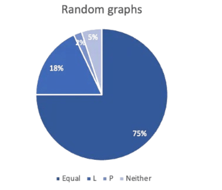
This means 75% of the time, all three outputted the same, 93% of the time we got the right result using the Laplacian method, 77% of the time we had a correct answer with just the Permanental, and 5% of the time we did not obtain a correct answer by either of the methods.

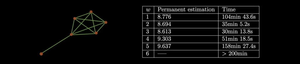
4. Boosting probabilities

Last but not least, boosting our results. Not only might post-selection reject a considerable portion of our samples, but the advantage to estimate permanents over classical approaches can be hard to verify. To soften this, to have a better run time and increase the prospects of seeing a practical quantum advantage, we studied how to better approximate the permanent with less samples. Put simply, we hack the adjacency matrix by multiplying the row corresponding to the least connected node by a number and encode the new matrix into the device; this might allow us to increase the probability, depending on the connectivity.

In the following table, we give some of the results over different w for the graph on the left.

Conclusion and final remarks

The applications and algorithms we developed were focused on graph problems, but the interesting fact is that our encoding method allows the encoding of any bounded matrix.

An important factor is the complexity of these algorithms. To estimate permanents by sampling, one obtains a polynomially close estimate of the permanent using a polynomial (efficient) number of samples³. This rules out the prospect that our algorithms present an exponential quantum-over-classical advantage, as polynomial-time classical algorithms like the Gurvits algorithm ¹³can also approximate permanents to polynomial precision. However, it leaves open the possibility that our techniques might present a practical advantage over their classical counterparts.

A final note is that when comparing quantum algorithms to classical ones, a factor which is becoming increasingly relevant is their energy cost. In terms of resources, Quandela’s Ascella QPU (12 modes and 6 photons) has the potential to be more energy efficient when compared to its classical counterparts.

References

1. S. Aaronson and A. Arkhipov, The computational complexity of linear optics (2011) pp. 333–342 ↩︎
2. P. R. Halmos, Normal dilations and extensions of operators, Summa Brasil. Math 2, 134 (1950) ↩︎
3. R. Mezher, A. Carvalho, S. Mansfield, arXiv:2301.09594v1 ↩︎
4. N. Heurtel, A. Fyrillas, et al., Perceval: A software platform for discrete variable photonic quantum computing, arXiv preprint arXiv:2204.00602 (2022) ↩︎
5. R. Mezher, A. Carvalho, S. Mansfield, arXiv:2301.09594v1 ↩︎
6. R. Mezher, A. Carvalho, S. Mansfield, arXiv:2301.09594v1 ↩︎
7. Nicolas Bourgeois, Aristotelis Giannakos, Giorgio Lucarelli, Ioannis Milis, Vangelis Paschos. Exact and approximation algorithms for densest k-subgraph. 2012. ⟨hal-00874586⟩ ↩︎
8. R. Mezher, A. Carvalho, S. Mansfield, arXiv:2301.09594v1 ↩︎
9. P. R. Halmos, Normal dilations and extensions of operators, Summa Brasil. Math 2, 134 (1950) ↩︎
10. R. Merris, K. R. Rebman, and W. Watkins, Permanental polynomials of graphs, Linear Algebra and Its Applications 38, 273 (1981) ↩︎
11. R. Mezher, A. Carvalho, S. Mansfield, arXiv:2301.09594v1 ↩︎
12. R. Merris, K. R. Rebman, and W. Watkins, Permanental polynomials of graphs, Linear Algebra and Its Applications 38, 273 (1981) ↩︎
13. L. Gurvits, in International Symposium on Mathematical Foundations of Computer Science (Springer, 2005) pp. 447–458. ↩︎